In our previous post, we manually implemented the Markov Chain Monte Carlo (MCMC) algorithm, specifically Metropolis-Hastings, to draw samples from the posterior distribution. The code isn’t particularly difficult to understand, but it’s also not very intuitive to read or write. Besides the challenges of implementation, algorithm performance (i.e., speed) is a major consideration in more realistic applications. Fortunately, well-optimized tools are available to address these obstacles, namely Stan and PyMC3.
Subjectively speaking, Stan is not my cup of tea. I remember spending an entire afternoon trying to install RStan, only to fail. To make matters worse, Stan has its own specialized language, adding another layer of complexity. In contrast, PyMC3 is much easier to install. The documentation and tutorials are well-written, and anyone with a basic understanding of Bayesian statistics should be able to follow them without much trouble. In this post—and future posts—I will stick with PyMC3.
Import modules
# if you haven't installed PyMC3 yet, simply do
# pip install pymc3
import matplotlib.pyplot as plt
import numpy as np
import pymc3 as pm
from pymc3 import *
import seaborn as sns
Data
This is the data we have been using so far.
x = np.array([5,3,4,6])
Build the model, Sampling from the posterior distribution
with Model() as model:
    # Define priors
    Poiss_lambda = Gamma("Poiss_lambda", alpha=2, beta=2)

    # Define likelihood
    likelihood = Poisson("x", mu =  Poiss_lambda, observed=x)

    # Inference
    trace = sample(3000, cores=2)  # draw 3000 posterior samples
Plot
plt.figure(figsize=(7, 7))
plot_trace(trace)
plt.tight_layout();
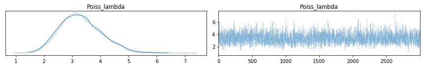
Notice that the picture is almost identical as what I drew before. On the left side, you see the density plot (which could be interpreted as a smooth histogram), where we can find the peak when \(\lambda \approx 3.2\). The right-hand side picture is simply a random walk of \(\lambda\), which can be used to determine if the sampling is stable.
Maximum A Posteriori
Of course we can use PyMC3 to find the parameters that give the maximum posteriori. The code is simple:
pm.find_MAP(model=model)
Unsurprisingly, we get:
{'Poiss_lambda_log__': array(1.15267951), 'Poiss_lambda': array(3.16666667)}
,which is the same as what we have calculated here
Posterior Predictive Distribution
To sample the posterior predictive distribution, type
# sampling
with model:
    ppc = pm.fast_sample_posterior_predictive(trace,var_names =["x"])

# draw histogram
sns.histplot(x=ppc["x"].flatten(), binwidth = 1)
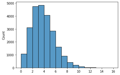
Again, the shape of the histogram is what we have seen before, which further validated our results.
Summary
So far we have covered the fundamentals of Bayesian inference, which includes topics like:
- Maximum A Posteriori
- Solve the denominator & Conjugate Prior
- Markov Chain Monte Carlo
- Posterior Predictive Distribution
- Probabilistic Programming - PyMC3
In the next few posts, I will switch gears and cover some other interesting topics like Hidden Markov Chain, Singular Value Decomposition, etc.
It will be fun, and stay tuned.