Introduction
This series of blog posts aims to explore the Hidden Markov Model (HMM) due to its broad applications across various fields, including natural language processing, population genetics, finance, and more. Beyond its practical utility, I find HMM particularly fascinating because it bridges multiple disciplines such as probability, linear algebra, machine learning, and computer science. In this post, I will introduce the Markov Chain, which serves as the foundation of HMM. As before, the concepts will be explained through a simple example, with minimal use of complex mathematical notation.
An example
Imagine there are only 100 people and three cities (New York, Boston, and Houston) in this world. Currently, 50 people live in New York, 30 people live in Boston, and 20 people live in Houston. Every year, a certain proportion of the population moves from one city to another, causing the population of each city to change constantly. Below is a diagram that shows the proportions:
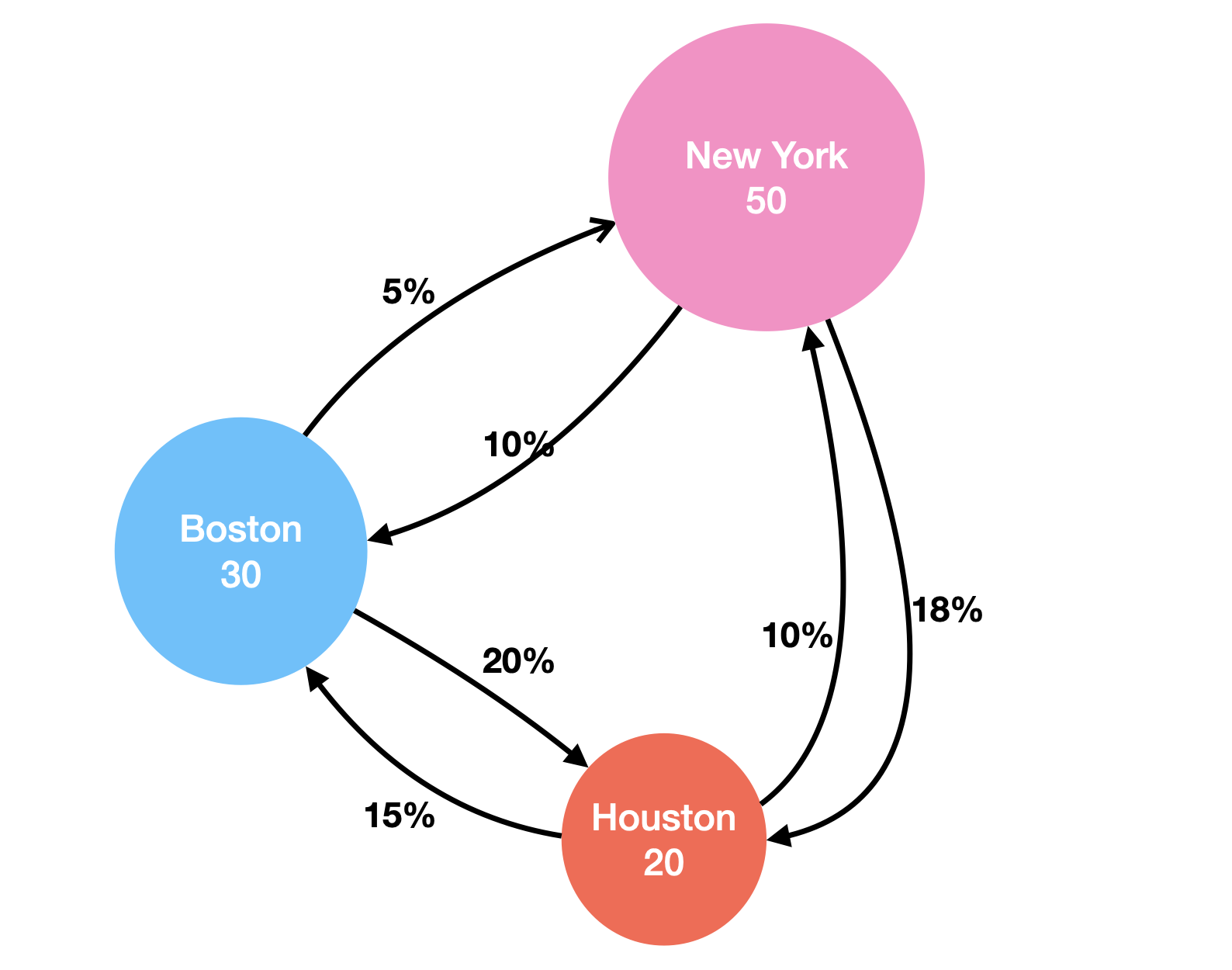
The question is: what is the population size for each city in the next year?
The question is trivial to solve with some algebra. For example:
For New York, next year, 5% of Boston’s population will move in, 10% of Houston’s population will move in, and 1 - 10% - 18% = 72% of New York’s population will remain in New York. So, in total, next year, New York will have:
$$ 0.72 \times 50 + 0.05 \times 30 + 0.1 \times 20 = 39.5 $$
Similarly, for Boston, we have: $$ 0.1 \times 50 + 0.75 \times 30 + 0.15 \times 20 = 30.5 $$
For Houston, we have:
$$ 0.18 \times 50 + 0.2 \times 30 + 0.75 \times 20 = 30 $$
To make the expression more compact, it’s helpful to rewrite these three linear equations into matrix form:
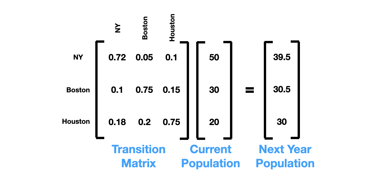
Besides being more compact, one advantage of using a matrix and vector representation is that it helps keeping track of the population of 2nd year, 3rd year, 4th year, etc.
For example, to calculate the population of the 2nd year, we simply multiply the matrix with the population of the previous year:
$$ \begin{bmatrix} 0.72 & 0.05 & 0.1 \\ 0.1 & 0.75 & 0.15 \\ 0.18 & 0.2 & 0.75 \end{bmatrix} \cdot \begin{bmatrix} 39.5 \\ 30.5 \\ 30 \end{bmatrix} = \begin{bmatrix} 33 \\ 31.3 \\ 35.7 \end{bmatrix} $$
To calculate the 3rd year, we have
$$ \begin{bmatrix} 0.72 & 0.05 & 0.1 \\ 0.1 & 0.75 & 0.15 \\ 0.18 & 0.2 & 0.75 \end{bmatrix} \cdot \begin{bmatrix} 33 \\ 31.3 \\ 35.7 \end{bmatrix} = \begin{bmatrix} 28.9 \\ 32.1 \\ 39 \end{bmatrix} $$
This is equivalent to $$ \begin{bmatrix} 0.72 & 0.05 & 0.1 \\ 0.1 & 0.75 & 0.15 \\ 0.18 & 0.2 & 0.75 \end{bmatrix}^3 \cdot \begin{bmatrix} 50 \\ 30 \\ 20 \end{bmatrix} = \begin{bmatrix} 28.9 \\ 32.1 \\ 39 \end{bmatrix} $$
,which is raising the matrix to the power of the year, and multiply by the initial population vector.
Stationary distribution
Believe it or not, the population of each city won’t change after many years, regardless of the initial population size of each city. We can show this by calculating the population after 20 years and after 50 years with different initial population size.
Here we use initial population vector \([50, 30, 20]\), and we calculate the population after 20 years:
$$ \begin{bmatrix} 0.72 & 0.05 & 0.1 \\ 0.1 & 0.75 & 0.15 \\ 0.18 & 0.2 & 0.75 \end{bmatrix}^{20} \cdot \begin{bmatrix} 50 \\ 30 \\ 20 \end{bmatrix} = \begin{bmatrix} 21.7 \\ 34.8 \\ 43.5 \end{bmatrix} $$
Here is the population after 50 years: $$ \begin{bmatrix} 0.72 & 0.05 & 0.1 \\ 0.1 & 0.75 & 0.15 \\ 0.18 & 0.2 & 0.75 \end{bmatrix}^{50} \cdot \begin{bmatrix} 50 \\ 30 \\ 20 \end{bmatrix} = \begin{bmatrix} 21.7 \\ 34.8 \\ 43.5 \end{bmatrix} $$
In a parallel universe, at year-0, we have 100 people in NY, 0 people in Boston, and 0 people in Houston. However, after 20 years, we achieve the same population across these three cities:
$$ \begin{bmatrix} 0.72 & 0.05 & 0.1 \\ 0.1 & 0.75 & 0.15 \\ 0.18 & 0.2 & 0.75 \end{bmatrix}^{20} \cdot \begin{bmatrix} 100 \\ 0 \\ 0 \end{bmatrix} = \begin{bmatrix} 21.7 \\ 34.8 \\ 43.5 \end{bmatrix} $$
It turns out that the population, after many years of migration, becomes independent of the initial population, and this is called a “stationary distribution.” This means the population of each city no longer changes over time. In fact, the stationary distribution is an intrinsic property of the matrix we have specified.
An Extra Note
In fact, the stationary distribution is the first eigenvector of the transition matrix!!!
(If the word “eigenvector” sounds unfamiliar, don’t worry about it. Intuition is more important here.)
(If it sounds familiar, try pulling out a calculator and calculating the first eigenvector, then rescale the vector so that the elements sum up to 1. This eigenvector should match with what we have computed above)
A trillion dollar model
In 1999, two Ph.D students at Stanford University named Larry Page and Sergey Brin developed a model that tried to recommend certain websites to users. The model was so successful that they even quit the Ph.D program. Years after, they became the most successful businessmen on earth, and the company they built is called Google.
The core idea of the webpage recommendation system is to recommend high quality websites. What is a high quality website? A high quality websites is a website that many websites referred to, (a.k.a: a website that has many hyperlinks pointed to). This assumption makes intuitive sense - an analogy is that a paper that has a lot citations must be a good paper. Based on this assumption, Page & Brin built this model called PageRank.
Assume there are 5 websites, and each arrow represents a hyperlink that goes from one page to another page:
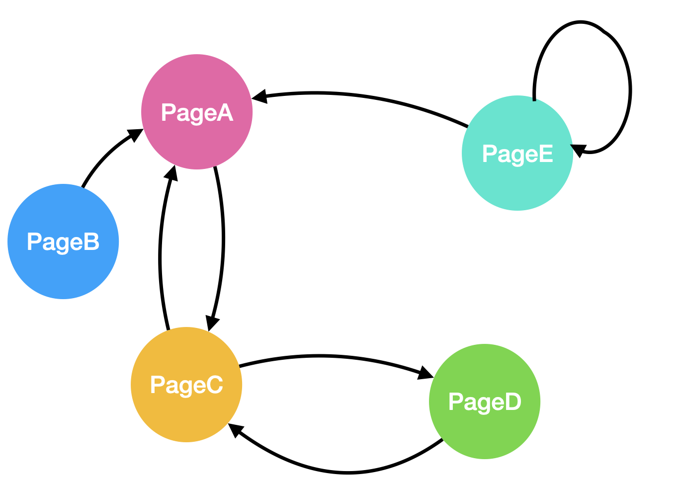
Intuitively, pageA and pageC look like good pages, since a lot of other websites referred these two pages. A user will typically follow the hyperlinks to browse the website. For example, if a user is currently browsing pageC, the next moment, this user will have 50% of the chance to go to pageD, and 50% of the chance to go to pageA. Based on this graph, we can specify the transition matrix
(note row/column order from pageA - pageE):
$$ \begin{bmatrix} 0 & 1 & 0.5 & 0 & 0.5\\ 0 & 0 & 0 & 0 & 0 \\ 1 & 0 & 0 & 1 & 0 \\ 0 & 0 & 0.5 & 0 & 0 \\ 0 & 0 & 0 & 0 & 0.5 \end{bmatrix} $$ Now assume we have 100 random users, with 20 users in each page. Using the same technique we have discussed above, we can calculate the stationary distribution (a.k.a, how many random users in each page eventually).
$$ \begin{bmatrix} 0 & 1 & 0.5 & 0 & 0.5\\ 0 & 0 & 0 & 0 & 0 \\ 1 & 0 & 0 & 1 & 0 \\ 0 & 0 & 0.5 & 0 & 0 \\ 0 & 0 & 0 & 0 & 0.5 \end{bmatrix}^{20} \cdot \begin{bmatrix} 20 \\ 20 \\ 20 \\ 20 \\ 20 \end{bmatrix} = \begin{bmatrix} 23.3 \\ 0 \\ 53.4 \\ 23.3 \\ 0 \end{bmatrix} $$
According to the PageRank algorithm, eventually we will have 53.4 users landing on pageC, and therefore pageC has the highest quality and should be recommended as the top page to the users.
(There are more interesting techniques Page & Brin used in this model. For example, how to prevent the random surfer from trapping in a certain loop, but this is beyond the scope of this post.)
In the next few posts, I will discuss HMM model in detail. Stay in tune!