In this post, I will show you THE most important technique in inferential statistics: Maximum Likelihood Estimation (MLE).
1. Some data to work with
Before we get started, let’s see what type of problem could be solved using MLE.
For example, I recorded the number of visitors of this website each hour from 8:00 am - 12:00 am (p.s. off course this is fake data, and I am probably too optimistic), and I hope to have a model that can accurately describe my data, and well as making predictions. Here is my data:
| Time | Number of visitors |
|---|---|
| 8:am - 9:am | 5 |
| 9:am - 10:am | 3 |
| 10:am - 11:am | 4 |
| 11:am - 12:am | 6 |
The first thing you need to do is to choose an appropriate probability distribution to describe your data. From your experience, you are happy with a poisson distribution, which has a probability mass function: $$f(x) = \frac{\lambda^x e^{- \lambda}}{x !}$$
where \(x\) is our observed data and \(\lambda\) the parameter we want to estimate.
(p.s. You can also use other distributions like negative binomial to model count data.)
2. Let’s experiment with different \(\lambda\)
Try \(\lambda = 2\).
The core question here is:
Assume \(\lambda = 2\), then what is the probability of observing our data?
That shouldn’t be difficult to answer. We first plug \(\lambda = 2\) into the probability mass function, and get: $$f(x) = \frac{2^x e^{- 2}}{x !}$$
Now we can calculate the probability of having exact 5 visitors in 1-hour duration. \(f(x = 5) = \frac{2^5 e^{- 2}}{5 !} = 0.036\)
Similarly, we have:
\(f(x = 3) = \frac{2^3 e^{- 2}}{3 !} = 0.18\)
\(f(x = 4) = \frac{2^4 e^{- 2}}{4 !} = 0.09\)
\(f(x = 6) = \frac{2^6 e^{- 2}}{6 !} = 0.012\)
Since our sample is independent and identically distributed (a.k.a. i.i.d), the probability of observing our data ( \([5,3,4,6]\) ) given \(\lambda = 2\), is simply the product of the probabilities we have calculated:
$$P(data | \lambda = 2) = 0.036 \times 0.18 \times 0.09 \times 0.012 = 7 \times 10^{-6}$$
Try \(\lambda = 4\)
The calculation is exactly the same, and I am not going to repeat this. But here is the result:
\(f(x = 5) = 0.156\)
\(f(x = 3) = 0.195\)
\(f(x = 4) = 0.195\)
\(f(x = 6) = 0.104\)
Again, we want to calculate the probability of observing those data, given \(\lambda = 4\):
$$P(data | \lambda = 4) = 0.156 \times 0.195 \times 0.195 \times 0.104 = 6.2 \times 10^{-4}$$
Notice the conditional probability in our example \(P(data | \lambda = \lambda_0)\), is also called likelihood function: \(L(\lambda = \lambda_0 | data)\)
Also notice that when we change \(\lambda\), the result of \(\prod_ip(x_i | \lambda)\) (a.k.a. likelihood) also change. In our example, when \(\lambda\) change from 2 to 4, our likelihood function increased. This means \(\lambda = 4\) is a superior model, as it better aligns with our observed data.
The goal of MLE is to find \(\lambda_0\) to maximize the likelihood of the observed data given the model.
3. Find \(\lambda_0\)
Now the question become clear, we have:
$$
L( \lambda| data) = P(data| \lambda) = f_{\lambda}(5) \times f_{\lambda}(3) \times f_{\lambda}(4) \times f_{\lambda}(6) \\
= \frac{\lambda^5 e^{- \lambda}}{5 !} \times \frac{\lambda^3 e^{- \lambda}}{3 !} \times \frac{\lambda^4 e^{- \lambda}}{4 !} \times \frac{\lambda^6 e^{- \lambda}}{6 !}
$$
And we are trying to find the \(\lambda_0\) to make sure the \(L( \lambda_0 | data)\) is the greatest. In mathematical notation:
$$ \underset{\lambda}{\mathrm{argmax}} (L( \lambda | data)) $$
Obviously, you can take the derivative of the likelihood function to find the maximum value, but this is beyond the scope of this blog. However, if you are interested, please check the appendix. I drew a graph to show you the relationship between \(\lambda\) and \(L( \lambda | data)\)
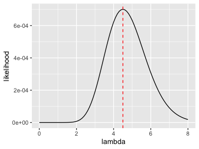
You can visually tell, when \(\lambda = 4.5\), our likelihood function reaches its maximum.
In fact, \(\lambda = 4.5\) is the average number of our data, and this is not a coincidence~
Summary
In summary, when we observed a set of data \([5,3,4,6]\) and we believed our data is from a poisson distribution, the “best guess” (under frequentist’s framework) of that poisson distribution is that it has \(\hat \lambda = 4.5\), which is the average of our data points.
That’s the end of this post Thanks for reading.
Appendix
We have the likelihood function:
$$ L(\lambda | data) = \frac{\lambda^5 e^{- \lambda}}{5 !} \times \frac{\lambda^3 e^{- \lambda}}{3 !} \times \frac{\lambda^4 e^{- \lambda}}{4 !} \times \frac{\lambda^6 e^{- \lambda}}{6 !} $$
Let $$g(\lambda) = \log(L(\lambda | data))$$
Taking the logarithm wouldn’t change the place where the function reach its peak. Therefore, we can instead find the \(\lambda\) that maximizes \(g(\lambda)\).
After applying logarithm, we have $$ g(\lambda) = \log(\frac{\lambda^5 e^{- \lambda}}{5 !} \times \frac{\lambda^3 e^{- \lambda}}{3 !} \times \frac{\lambda^4 e^{- \lambda}}{4 !} \times \frac{\lambda^6 e^{- \lambda}}{6 !}) $$
Since logarithm covert product to summation, we have:
$$ g(\lambda) = [\log(\lambda ^5) - \lambda - \log(5!) ]+ [\log(\lambda ^3) - \lambda - \log(3!)] \\\ + [\log(\lambda ^4) - \lambda - \log(4!)]+[\log(\lambda ^6) - \lambda - \log(6!)] $$
We then take the derivative of \(g(\lambda)\):
$$ g(\lambda)’ = \frac{5}{\lambda} - 1 + \frac{3}{\lambda} - 1 + \frac{4}{\lambda} - 1 +\frac{6}{\lambda} - 1 $$
Let \(g(\lambda)' = 0\), we have:
$$ \frac{5}{\lambda} - 1 + \frac{3}{\lambda} - 1 + \frac{4}{\lambda} - 1 +\frac{6}{\lambda} - 1 = 0 $$
Solve \(\lambda\), we have:
$$ \lambda = 4.5 $$