How to draw sample from a generic distribution?

In this post, I am going to show two methods to draw samples from a generic distribution.

But before we get started, we should define what do I mean generic distribution. Here is one example:

$$ f(x)= \begin{cases} 0 & \text{if $x$ < 0} \\ c \cdot \sqrt{x} & \text{if $0 < x < 1 $} \\ 0 & \text{if $x > 1$} \end{cases} $$

First, let’s take a look at the probability density function (pdf):

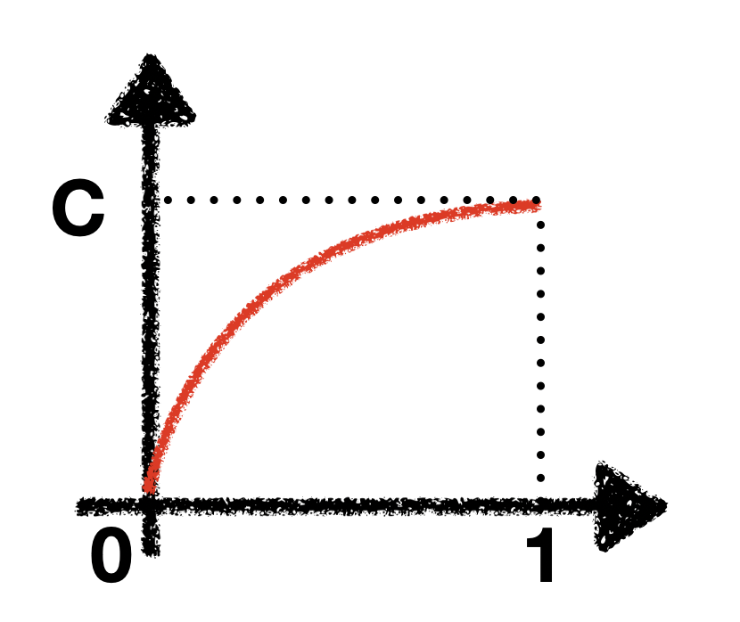
Obviously, this is not any type of distribution we have learned before (not Gaussian, not Poisson, not uniform etc), and therefore, we wouldn’t be able to use build-in functions to draw samples from (in R programming language, we have rnorm(), rpois(), runif()).

Despite the limitations, there are still ways to draw samples from, which I will discuss below:

Method 1: inverse transform sampling

You may have noticed that our function has a constant $c$. In order for this curve to be a legit probability density function, we have to make sure that the area under the curve is 1. In mathematical notation, we have $$ \int_{0}^{1} c \sqrt{x} = 1 $$

Finding the integral isn’t difficult. We have $$ F = \frac{2c}{3} \cdot x^{1.5} $$

We have to make sure $F |_{0}^{1} = 1$, therefore we solve $c = 1.5$

Plug $c = 1.5$ into our pdf and cdf, we pdf:

$$ f(x)= \begin{cases} 0 & \text{if $x$ < 0} \\ 1.5 \cdot \sqrt{x} & \text{if $0 < x < 1 $} \\ 0 & \text{if $x > 1$} \end{cases} $$

And we have cdf:

$$ cdf(x)= \begin{cases} 0 & \text{if $x$ < 0} \\ x^{1.5} & \text{if $0 < x < 1 $} \\ 1 & \text{if $x > 1$} \end{cases} $$

The steps I described above are pretty standard and boring, but here comes to the interesting part that allows us to sample from this generic distribution.

Step1: Inverse the cdf

We first find the inverse of cumulative density function. $x = y^{2/3}$

Step2: Sampling

We draw sample y from a uniform distribution, then raise this sample to the power of $2/3$, and we will get a customized sampler!

Sampler <- function(n = 1){
     y = runif(n, min = 0, max = 1)
     x = y ^(2/3)
     return(x)
}

# draw one sample 
Sampler()
## [1] 0.6835192


# draw 10000 samples
hist(Sampler(10000), probability = T, main = "Histogram, inverse transform sampling")
lines(seq(0,1, 0.01), 1.5 * sqrt(seq(0,1, 0.01)), col = "red" )

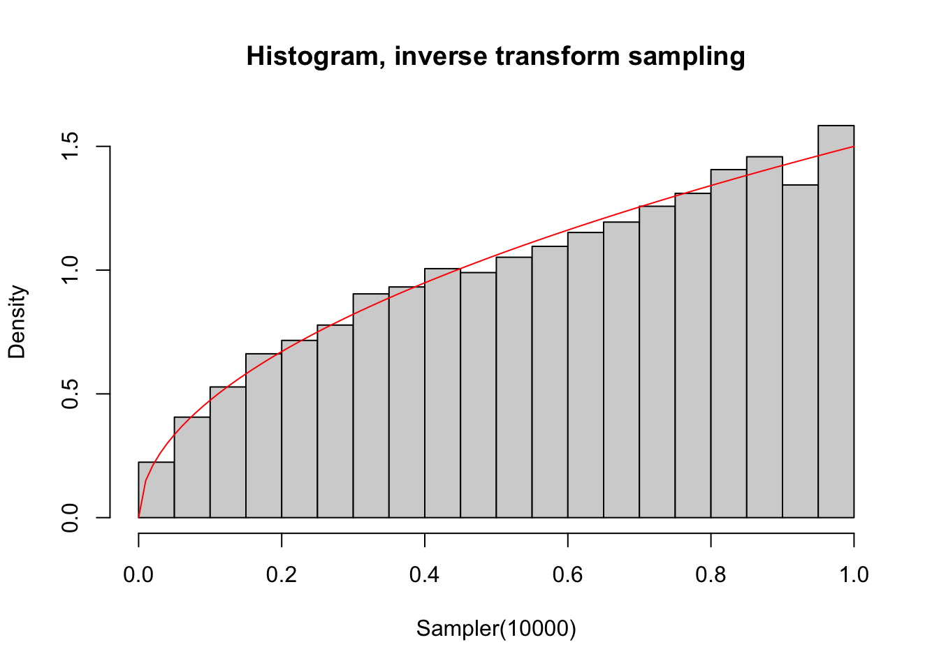
The red line represents the theoretical pdf, and it perfectly matches this histogram!

Method 2: accept-reject sampling.

This is a trick that allows you to draw samples without explicitly calculating $c$. It is particularly useful if it’s difficult to normalize the probability (e.g. Bayesian statistics).

Here are the steps involved:

Step1: Find an easy-to-sample distribution $g(x)$ (normal, uniform, etc) and multiply by a constant $k$, so that $k \times g(x)$ is always greater than our customized distribution $f(x)$.
Step2: Draw a sample from $g(x)$
Step3: Calculate the probability of acceptance: $p (accept) = \frac{f(x)}{k \cdot g(x)}$
Step4: Collect samples. The bag of your collected samples will have a distribution of $f(x)$.

Notice that you don’t need the full format of f(x). In our case, you can ignore $c$, and set $f(x) = \sqrt x$

# our collecting bag
accept = c()

# draw 100000 samples from a uniform distribution
samples = runif(100000, 0, 1)

# iterate all the samples
for (sample in samples){
   accpt_prob = sqrt(sample)/(2 * 1)           # calculate the probability of acceptance
    if (rbinom(n = 1, size = 1, prob = accpt_prob) == 1){ # flip a unfair coin with probability we just calculated. If head up, we accept.
        accept = c(accept, sample)               # add the accepted samples to our bag
    }
}

# draw 10000 samples
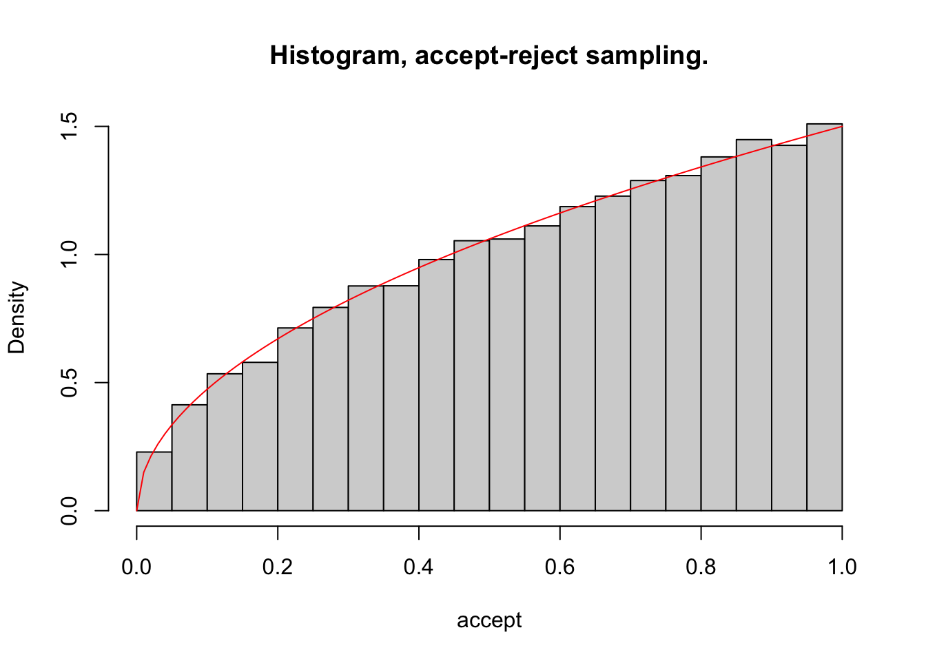
hist(accept, probability = T, main = "Histogram, accept-reject sampling.")
lines(seq(0,1, 0.01), 1.5 * sqrt(seq(0,1, 0.01)), col = "red" )


# proportion of samples accepted
length(accept)/100000
## [1] 0.33196

Notice here, I chose the constant $k = 2$. We are sure that $2 \times U(0, 1)$ is always larger than our customized pdf.

Also, notice in my code, I use $f(x) = \sqrt x$, but not $f(x) = 1.5 \sqrt x$, although either way works.

You might find that I drew 100000 samples, but only a small proportion of samples are accepted. This is one of a big disadvantage of accept-reject sampling!

Being able to draw samples without knowing its full format is very advantageous. This accept-reject sampling is a core foundation of MCMC sampling, which I will demonstrate in the next few posts

Summary

In this post, we learned two ways of drawing samples form a customized distribution. Either one has its pros and cons.

Method	Advantage	Disadvantage
Inverse Transform Sampling:	Utilizes all the samples	Need to calculate cdf; Inverse cdf sometimes could be very difficult
Accept Reject Sampling:	Do not require full format of pdf, easy to implement	Waste samples

Reference:

ritvikmath: https://www.youtube.com/watch?v=OXDqjdVVePY
Ben Lambert: https://www.youtube.com/watch?v=rnBbYsysPaU