Calculate PCA by hand (via eigen-decomposition)

In this blog post, I will calculate PCA step-by-step (via eigen-decomposition).

But before we dive deep into PCA, there are two prerequisite concepts we need to understand:

• Variance/Covariance
• Find eigenvectors and eigenvalues

If you already familiar those two concepts, feel free to skip those sections.

 
 
 
 

Prerequisite 1: Variance/Covariance

Variance

Variance measures how far a set of numbers is spread out from their average value. The sample variance is defined as:

$$s^2 = \frac{\sum(x_i - \bar x)^2}{n - 1}$$

Let’s say you have a vector $\vec{v} = [1, 2,3 ]$. To calculate the variance, there are two steps:

• Calculate mean: $\bar v = \frac{(1 + 2 + 3)}{3 } = 2$
• Calculate variance: $s^2 = \frac{(1 - 2)^2 + (2 - 2)^2 + (3 - 2)^2}{3 -1} = 1$

 
 

Covariance

The covariance of two vector $\vec{x}, \vec{y}$ is defined as $$Cov(x,y) = \frac{\sum{(x_i - \bar x)(y_i - \bar y)}}{n - 1}$$ If the $Cov(x, y) > 0$, that means $\vec{x}, \vec{y}$ have the same trend (they co-increase or co-decrease).
If the $Cov(x, y) < 0$, that means $\vec{x}, \vec{y}$ have the opposite trend (one increases, the other decreases).

Let’s give an example here. $$\vec{x} = [1,2,3], \vec{y} = [3,2,7]$$

To calculate the covariance, we have two steps as well:

• Calculate the mean of $\vec{x}, \vec{y}$. We have $\bar x = 2$, $\bar y = 4$
• Calculate the covariance $Cov(x, y) = \frac{(1 - 2) \cdot (3 - 4) + (2 - 2) \cdot (2 - 4) + (3 - 2) \cdot (7 - 4)}{3 - 1} = 2$.

Since the $Cov(x, y) = 2 > 0$, we know that $\vec{x}, \vec{y}$ co-vary.

If we plot those three points in a x-y coordinate plane, we get:

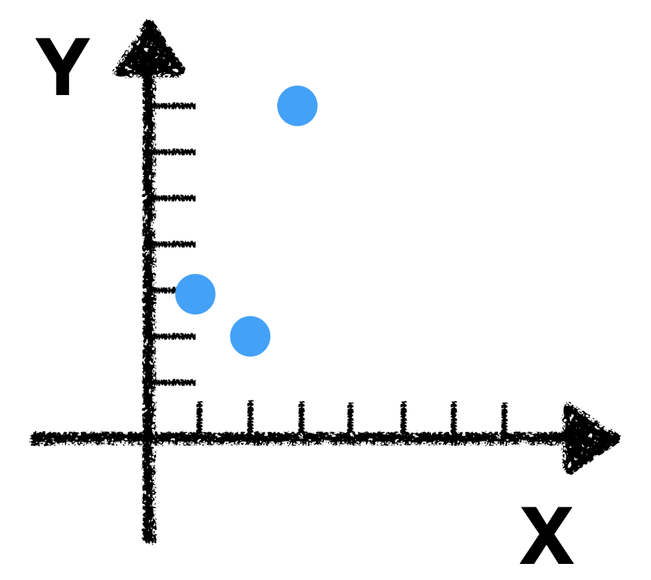
It is obvious that $\vec{x}, \vec{y}$ have the same trend (they go up/down together).

 
 
 
 

Prerequisite 2: Find eigenvectors and eigenvalues

The word “eigen” sounds scary, at least to me when I first learned linear algebra. But it is not that complicated. I am going to walk you through the calculation of eigenvalue and eigenvectors.

Assume you have a matrix $\mathbf{A}$, all eigen-decomposition does is that it finds a set of vectors $\vec{v}$ and $\lambda$, so that $$\mathbf{A } \cdot \vec{v} = \lambda \vec{v}$$

This means applying a linear transformation $\mathbf{A}$ to the vector $\vec{v}$, is the same as scaling $\vec{v}$ by a factor $\lambda$. In other word, the linear transformation(a.k.a matrix) $\mathbf{A}$ doesn’t rotate $\vec{v}$.

 

Here I provide an example with a $2 \times 2$ matrix. Let’s say our matrix $\mathbf{A}$ is:

$$\begin{bmatrix} 0 & -1 \\ 2 & 3 \end{bmatrix}$$

By definition, we want to find $\vec{v}, \lambda$ so that $$\begin{bmatrix} 0 & -1 \\ 2 & 3 \end{bmatrix} \cdot \vec{v} = \lambda \vec{v}$$

We find $\lambda$ first. Let the right side of the equation times the identity matrix $\mathbf{I}$,

$$\begin{align} \begin{bmatrix} 0 & -1 \\ 2 & 3 \end{bmatrix} \cdot \vec{v} &= \lambda \cdot \begin{bmatrix} 1 & 0 \\ 0 & 1 \end{bmatrix} \cdot \vec{v} \\ \begin{bmatrix} 0 & -1 \\ 2 & 3 \end{bmatrix} \cdot \vec{v} &= \begin{bmatrix} \lambda & 0 \\ 0 & \lambda \end{bmatrix} \cdot \vec{v} \\ \begin{bmatrix} 0 - \lambda & -1 \\ 2 & 3 - \lambda \end{bmatrix} \cdot \vec{v} &= \vec{0} \\ det ( \begin{bmatrix} 0 - \lambda & -1 \\ 2 & 3 - \lambda \end{bmatrix} ) &= 0 \\ -\lambda \cdot (3 - \lambda) + 2 &= 0 \end{align}$$

Solve this quadratic equation, we get: $\lambda_1 = 2$, $\lambda_2 = 1$.

 

So far we have found our eigen-values ( $\lambda$ ). The next step is to find our eigenvectors. We should have $\vec{v_1}, \vec{v_2}$, each of them is paired with an eigenvalue. Also, notice that there are infinite amount of eigenvectors and they all point to the same direction. We want to find the one with length equal to 1.

 
To calculate eigenvectors, we simply plug $\lambda_1, \lambda_2$ into the following equation, which is obtained when we are trying to figure out eigenvalues:

$$\begin{bmatrix} 0 - \lambda & -1 \\ 2 & 3 - \lambda \end{bmatrix} \cdot \vec{v} = \vec{0}$$

We plug in $\lambda_1 = 2$, and get

$$\begin{bmatrix} -2 & -1 \\ 2 & 1 \end{bmatrix} \cdot \vec{v_1} = \vec{0}$$

This is essentially finding the null space of the matrix on the left side. I will skip this part for now, but you can find plenty of resources online. But here is the result: $\vec{v_1} = [0.447, -0.894]$.

 

We can apply the same technique to find the second pair of eigenvalue & eigenvector:

$\lambda_2 = 1, \vec{v_2} = [-0.707, 0.707]$

 
 
 
 
 
 

PCA: eigen-decompose the covariance matrix

If you are still with me, you are 80% done. The rest of this post is simply combine the two techniques I discussed above.

Let’s say we have a matrix ` $$\begin{bmatrix} 1 & 0 \\ 0 & 1 \\ -1 & -1 \end{bmatrix}$$

Generally, each row represents our observations/samples, and each column represents features we measured. After applying PCA, we are expect to reduce the dimensionality of the matrix, while still retain most of the information.

Keep in mind, the high level intuition of PCA is that you rotate the coordinate system, so that your first coordinate (PC1) captures most of the variation, and second coordinate (PC2) captures the second most of the variation, etc…

Okay, let’s first take a look of our data

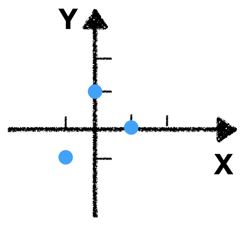
Imagine you fix the origin, and counterclockwise spin the coordinate system, until the x-axis capture the most of the variation. Here is a visual demonstration

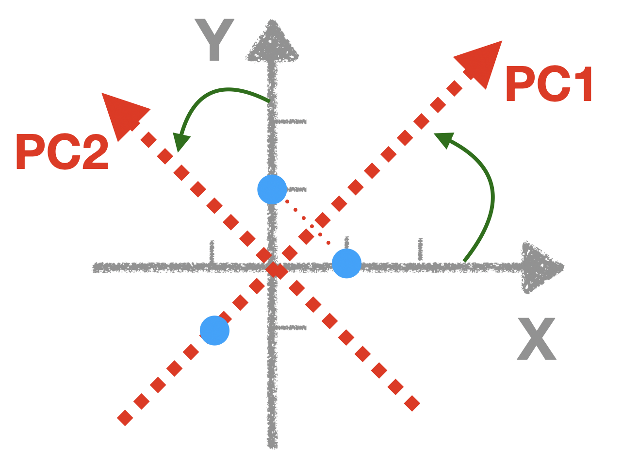
Now we can visually tell we should rotate 45 degree, so that our PC1 can capture most of the variation. But how can I calculate this mathematically?

 
 
 
 

Step 1

We have two features/columns $C1 = [1, 0, -1]$, $C2 = [0, 1, -1]$. Now we need to construct a matrix, where the diagonal entries are the variance, and off-diagonal entries are covariance. In our case, we should construct a matrix like this:

` $$\begin{bmatrix} Var(C1) & Cov(C1, C2) \\ Cov(C2, C1) & Var(C2) \end{bmatrix}$$

Use the technique (section 1) I described above, we have $$Var(C1) = 1$$ $$Var(C2) = 1$$ $$Cov(C1, C2) = Cov(C2, C1)= 0.5$$

Plug in the result, we have our covariance matrix: ` $$\begin{bmatrix} 1 & 0.5 \\ 0.5 & 1 \end{bmatrix}$$

 

Step 2

Find the eigenvalues and eigenvectors of our covariance matrix. We have

$$\lambda_1 = 1.5, \vec{v_1} = [0.707, 0.707]$$

$$\lambda_2 = 0.5, \vec{v_2} = [-0.707, 0.707]$$

Notice $\vec{v_1}$ is pointing to 45 degree upward, $\vec{v_2}$ is pointing to 135 degree upward, which is exactly what we expected.

Therefore, we find our $PC1$ and $PC2$, which are $\vec{v_1}$ and $\vec{v_2}$!

 

Step3

Here we can combine the eigenvectors into a matrix, with the first column to be $\vec{v_1}$, and second column to be $\vec{v_2}$. This is often called loading matrix (although the word “loading” is somewhat ambiguous) $$\begin{bmatrix} 0.707 & -0.707 \\ 0.707 & 0.707 \end{bmatrix}$$

If we multiply the loading matrix and our dataset, we should get our scores matrix, which is the projection of the data on the PCs.

$$\begin{bmatrix} 1 & 0 \\ 0 & 1 \\ -1 & -1 \end{bmatrix} \begin{bmatrix} 0.707 & -0.707 \\ 0.707 & 0.707 \end{bmatrix} = \begin{bmatrix} 0.707 & -0.707 \\ 0.707 & 0.707 \\ -1.414 & 0 \end{bmatrix}$$

 

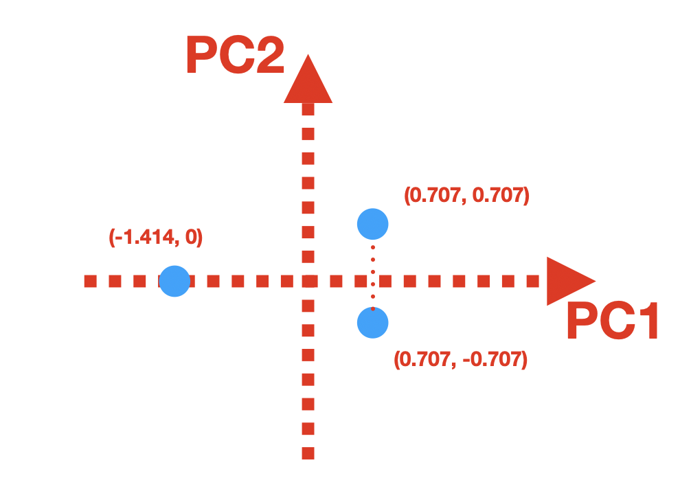
Now we have our transformed data: $$\begin{bmatrix} 0.707 & -0.707 \\ 0.707 & 0.707 \\ -1.414 & 0 \end{bmatrix}$$

Let’s plot our transformed data, with PCs be the coordinate system:

The last point here:

In the scores matrix, if you calculate the variance of the first column, you will get $Var(PC1) = 1.5$. For the second column, you will get $Var(PC2) = 0.5$.

Does the number look familiar? In fact, $$Var(PC1) = 1.5 = \lambda_1$$ $$Var(PC2) = 0.5 = \lambda_1$$

For this dataset, $\lambda_1$ explains 75% of the variance since $\frac{1.5}{1.5 + 0.5} =0.75$; Likewise, $\lambda_2$ explains 25% of the variance since $\frac{0.5}{1.5 + 0.5} =0.25$

In summary, eigenvalue tells you how much variance captured by its associated PC

 
 
 

That’s the end of this post. Thanks for reading!