Bayesian regression method for polygenic score
Polygenic score (PRS) investigates the genetic liability of certain diseases. Given the training data, we might compute the polygenic score as \(PRS_i = \sum_{j = 1}^{M} \hat \beta_j G_{ij}\) for the testing cohort. Most of the PRS methods paper, such as PRS-CS, LDPred aim to recover causal effects \(\lambda\) from the observed marginal effect size estimates \(\hat \beta_j\). Here let’s consider a infinitesimal model (LDpred-inf).
We assume the causal effect size \(\lambda \sim MVN(0, \frac{h^2}{M}I)\) (called infinitesimal model). From this post, we also have \(\hat \beta | \lambda \sim MVN(R \lambda, \frac{1 - h^2}{N}R)\). The Bayesian inference recipe with conjugate prior normal distribution gives us (according to this document ):
$$
\begin{split} p(\lambda \mid \hat \beta) &\propto f(\hat \beta \mid \lambda) \cdot f(\lambda) \\ &\propto \exp \{ - \frac{1}{2} (\hat \beta - R\lambda )^T (\frac{1 - h^2}{N}R)^{-1} (\hat \beta - R\lambda ) \} \cdot exp \{ - \frac{1}{2}\lambda^T (\frac{h^2}{M})^{-1} \lambda \} \\ &\propto \exp\{ - \frac{1}{2}[\frac{N}{1 - h^2}\cdot (\hat \beta - R\lambda )^T R^{-1}(\hat \beta - R\lambda ) +\frac{M}{h^2} \lambda^T \lambda ] \} \\ &\propto \exp \{- \frac{1}{2} [\frac{N}{1 - h^2} \cdot (\hat \beta^T R^{-1} \hat \beta - \hat \beta^T R^{-1} R \lambda -\lambda^T R R^{-1}\hat \beta + \lambda^T RR^{-1}R\lambda) + \frac{M}{h^2} \lambda^T \lambda] \} \\ &\propto \exp \{- \frac{1}{2} [\lambda^T(\frac{N}{1 - h^2}R + \frac{M}{h^2} I)\lambda - 2 \frac{N}{1 - h^2} \hat \beta^T \lambda ] \} \end{split}
$$
Let \(K = \frac{N}{1 - h^2}R + \frac{M}{h^2} I\), \(b = \frac{N}{1 - h^2} \hat \beta\), and use the “Completing the square” technique, we have:
$$
\begin{split} p(\lambda \mid \hat \beta) &\propto f(\hat \beta \mid \lambda) \cdot f(\lambda) \\ &\propto exp \{ (\lambda -K^{-1}b)^T K (\lambda -K^{-1}b) \} \end{split}
$$
Therefore, the posterior distribution of the causal effect size is
$$
\begin{split} \lambda \mid \hat \beta &\sim MVN(K^{-1}b, K^{-1}) \\ &\sim MVN((R + \frac{M(1 - h^2)}{Nh^2} I)^{-1} \hat\beta, [\frac{N}{1 - h^2}R + \frac{M}{h^2} I]^{-1}) \end{split}
$$
One might claim that the heritability of a region is small enough, such that \(1 - h^2 \approx 1\), Therefore, we can further simplify the expression, and obtain the mean and variance of the posterior causal effect size:
$$
\begin{split} \mathbb{E}[\lambda \mid \hat \beta ] &= (R + \frac{M}{Nh^2} I)^{-1} \hat\beta \\ \mathbb{V}ar[\lambda \mid \hat \beta ] &= [NR + \frac{M}{h^2} I]^{-1} \end{split}
$$
This expression is identical to what’s mentioned in PRS-CS paper (equation 13). But I have a few more remarks about this model:
-
In both PRS-CS and LDpred manuscript, they have an additional subscript to denote a small region of the genome (in PRS-CS, LD is denoted as
\(D_l\)to indicate the\(l\)-th region). This is because LD panel is pre-computed in blocks realistically. -
This approach attempts to solve a Bayesian inference problem without looking at individual-level data.
-
This infinitesimal Bayesian regression approach is identical to Ridge regression.
-
The heritability
\(h^2\)is treated as a parameter for the prior distribution, which must be specified according to domain knowledge before we run this analysis. This is not always trivial in realistic PRS analysis. Therefore, when we don’t have any prior information about a disease, we might try grid search to find the best\(h^2\). In machine learning lingo, this is referred as “hyper-parameter” tunning.
The framework can be further extended to multi-ancestry setting. Let’s assume that we have the same causal effect sizes \(\lambda\) across ancestries. For each ancestry \(k\), we have \(\hat \beta_{k} | \lambda \sim MVN(R_k \lambda, \frac{1}{N}R_k)\). We might infer the posterior effect size \(f(\lambda\mid \hat \beta_1, \hat\beta_2, ...)\):
$$
\begin{split} f(\lambda\mid \hat \beta_1, \hat\beta_2, ...) &\propto f(\beta_1, \hat\beta_2, ... \mid \lambda) \cdot f(\lambda) \\ &\propto \prod_{k = 1} f(\hat \beta_k \mid \lambda) \cdot f(\lambda) \end{split}
$$
It’s possible to expand the equation to find the posterior mean of \(\lambda \mid \hat \beta_1, \hat \beta_2...\), which would be a function of the prior distribution of \(\lambda\), observed effect sizes, and LD panel for each ancestry. However, this might not be a reasonable assumption about the prior distribution of \(\lambda\), as it might be different across populations (or heritability might be different, which implies different amount of regularization). PRS-CSx instead infers the posterior effect size for each ancestry.
Simulation
path = "https://www.mv.helsinki.fi/home/mjxpirin/GWAS_course/material/APOE_1000G_FIN_74SNPS."
haps = read.table(paste0(path,"txt"))
info = read.table(paste0(path,"legend.txt"),header = T, as.is = T)

n = 1000
G = as.matrix(haps[sample(1:nrow(haps), size = n, repl = T),] + haps[sample(1:nrow(haps), size = n, repl = T),])
row.names(G) = NULL
colnames(G) = NULL

G_ = scale(G)
h2 = 0.05
M = ncol(G_)
lambda = rnorm(ncol(G_), mean = 0, sd = sqrt(h2/M))

err = rnorm(n, mean = 0, sd = sqrt(1 - h2))


y = G_ %*% lambda + err
y_ = scale(y)

##
beta_hat = t(G_) %*% y / n
R = t(G_) %*% G_ /n # LD matrix


lambda_posterior = solve(R + M/(n *h2) * diag(M)) %*% beta_hat
plot(beta_hat, lambda_posterior, main = "GWAS effect sizes vs posterior effect sizes",
     xlim = c(-0.1, 0.1), ylim = c(-0.05, 0.05), xlab = "GWAS effect size (marginal)", ylab = "Posterior mean of lambda")
abline(a = 0, b = 1, col = "red")
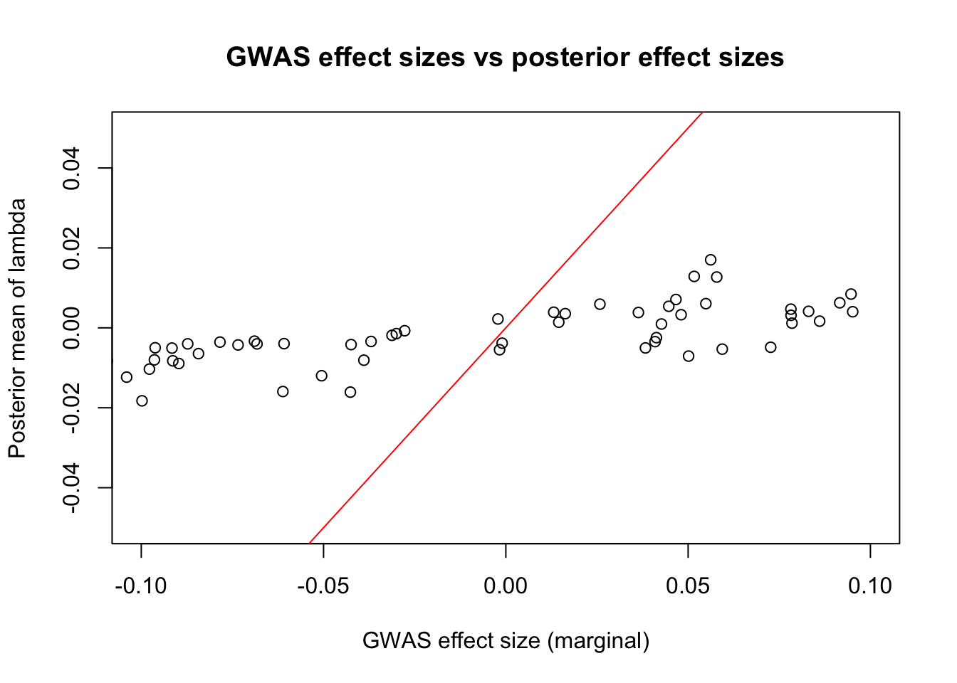
Clearly, there is a strong shrinkage of the marginal effect size.