Dive into Bayesian statistics (3): Markov Chain Monte Carlo

In this post, I will continue to use the same example that I used before (Bayesian: MAP and Bayesian: solve denominator). Also, it will be very helpful to first understand accept-reject sampling that I discussed in this post.

Now let’s get started!

As we discussed at the end of this post, solving the denominator is a non-trivial work, especially when you have many parameters to estimate. One way to overcome this obstacle is to use a method called Markov Chain Monte Carlo (MCMC).

The high level idea of MCMC is that although calculating the denominator is often unfeasible, we can still draw samples from the target distribution, even though we do not know the denominator (similar to the idea of accept reject sampling we discussed here).

In this post, I will introduce a popular method of MCMC called Metropolis-Hastings algorithm. The goal of this post is to show you the steps of Metropolis-Hastings algorithm, and to implement the algorithm in R. I won’t discuss the mathematical proof of why this algorithm works (because I do not understand neither), but show you the algorithm step by step.

Metropolis algorithm

Step1: Choose a distribution that is easy to sample from. Here we choose a normal distribution (set $\sigma = 1$).

Step2: Draw a sample $x_i$ form the normal distribution with $\mu = x_{i -1}, \sigma = 1$. Let’s call this sample “proposed sample”

Step3: Calculate the probability of acceptance $p = \frac{f(x_i)}{f(x_{i - 1})}$, where $f(x)$ is the target distribution (without knowing the denominator).

Step4: If $p > 1$, simply accept the proposed distribution.

Step5:

• Step5.1: If $p < 1$, flip an unfair coin with probability of heads to be $p$

• Step5.2: If we get a head from the coin, we accept the proposed sample.

• Step5.3: If we get a tail from the coin, we reject the proposed sample, but we duplicate the last accepted sample

Step6: Repeat this process many many times.

R code implementation

If you are like me, reading all those words might not make any sense. So let’s take a look the implementation. Again we will use the posterior distribution we calculated here:

$$ P(\lambda | \text{data}) = c \cdot \lambda^{19} e^{- 6 \lambda} \quad \text{, where $c$ is a constant.} $$

First, we need to express the posterior in R code. Notice when $\lambda < 0$, we explicitly set $f(\lambda) = 0$. Also, we ignored the constant $c$ in our expressions.

Again, this is our target distribution $f(x)$, and the goal is to draw samples from this distribution

# define the posterior distribution
posterior <- function(lambda){
  if (lambda > 0){
    return(lambda^19 * exp(-6*lambda))
  } else {
    return(0)
  }
}

Now let’s implement the Metropolis algorithm. Notice I use a vector called bag to collect all the samples:

# we need a place to start with, I set 8
bag = c(8)

# Metropolis algorithm
for(i in 2:5000){
  proposed = rnorm(1, mean= bag[i-1])    # propose a sample from the standard distribution
  prob = posterior(proposed)/posterior(bag[i-1])    # calculate the probability of acceptance 
  
  if (prob > 1){
    bag[i] = proposed     # if probability is greater than 1, we accept the proposed sample
  } else {
    coin = rbinom(1, size = 1, prob = prob)  # flip an unfair coin  
    if (coin == 1){
      bag[i] = proposed    # if the coin turned out to be head, we accept the proposed sample
    } else {
      bag[i] = bag[i-1]    # if the coin turned out to be tail, we duplicated the last accepted sample
    }
  }
}

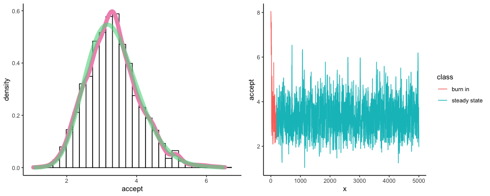
Here is what the result looks like.

On the right hand side plot, we simply connect all the dots in the vector bag. I used ggplot to draw this, but you can also draw this with plot(accept, "l").

Notice at the very beginning, our samples have large values (6~8), but then it drops to a smaller value and stay relatively stable. The samples we collected at the beginning is called “burn in period”, which means the Markov Chain hasn’t reached to a steady state, and these samples aren’t representative and should be discarded.

 
On the left hand side plot, I threw away the first 200 “burn in” samples, and drew a density histogram for the rest of my samples (you can draw this by tying hist(accept[201:5000])). The red line is the density line from our data. The green line is the theoretical probability density function of $\text{Gamma}(\alpha = 20, \beta = 6)$.

You can see the density line is very similar to our ground truth (the green line, which we have calculated here), which proves that our Metropolis algorithm indeed works.

Summary:

In this series of posts, we started from Maximum likelihood estimation, then incorporate a Gamma prior distribution and use various methods (integration, conjugate prior, and MCMC) to infer the posterior distribution. I hope this series of posts really helps you step into the door of Bayesian inference. If you like this post, simply drop a thumb up, and leave some comments.

Reference:

ritvikmath: https://www.youtube.com/watch?v=yApmR-c_hKU

ritvikmath: https://www.youtube.com/watch?v=yCv2N7wGDCw