Calculate SVD by hand (and decompose Spongebob)

2021-11-22 1700 words 8 minutes

Contents

In my previous post, I have manually implemented PCA by finding the eigenvectors and eigenvalues of a covariance matrix. Today, let’s try to perform PCA using a different approach called Singular Value Decomposition. Then we are going to decompose SPONGEBOB!

Note: you might find this post to be useful, if you are new to PCA.

Algorithm

Again, we are going to use the same dataset we have used before.

$$ \mathbf{ M} = \begin{bmatrix} 1 & 0 \\ 0 & 1 \\ -1 & -1 \end{bmatrix}$$

The formula of SVD stands: $$ \mathbf{ M} = \mathbf{ U \cdot \Sigma \cdot V ^{T}} $$

$\mathbf{ U }$ is the eigenvectors of $ \mathbf{ M \cdot M^T}$,

$\mathbf{ V }$ is the eigenvectors of $ \mathbf{ M^T \cdot M}$.

$\mathbf{ \Sigma }$ is a diagonal matrix with singular values (a.k.a square root of eigenvalues) of $ \mathbf{ M^T \cdot M}$.

Calculation:

(Note: I have discussed how to find eigenvectors and eigenvalues for a matrix in this post, and I will skip the steps for simplicity)

1. Calculate $\mathbf{ U }$

$$ \mathbf{ M \cdot M^T} = \begin{bmatrix} 1 & 0 \\ 0 & 1 \\ -1 & -1 \end{bmatrix} \cdot \begin{bmatrix} 1 & 0 & -1 \\ 0 & 1 & -1 \end{bmatrix} = \begin{bmatrix} 1 & 0 & -1 \\ 0 & 1 & -1 \\ -1 & -1 & 2 \end{bmatrix}$$

We then find the eigenvectors of $ \mathbf{ M \cdot M^T}$, and get

$$ \lambda_1 = 3, \mathbf{v_1} = [-0.408, -0.408, 0.816] \\ \lambda_2 = 1, \mathbf{v_2} = [0.707, -0.707, 0] \\ \lambda_3 = 0, \mathbf{v_3} = [0.577, 0.577, 0.577] $$

We write the eigenvectors into a matrix, with each column to be a eigenvector. Therefore, we have $$ \mathbf{U} = \begin{bmatrix} -0.408 & 0.707 & 0.577 \\ -0.408 & -0.707 & 0.577 \\ 0.816 & 0 & 0.577 \end{bmatrix} $$

2. Calculate $\mathbf{ V }$

The calculation is almost identical, we simply find the eigenvectors and eigenvalues of $ \mathbf{ M^T \cdot M}$

$$ \mathbf{ M^T \cdot M} = \begin{bmatrix} 1 & 0 & -1 \\ 0 & 1 & -1 \end{bmatrix} \cdot \begin{bmatrix} 1 & 0 \\ 0 & 1 \\ -1 & -1 \end{bmatrix} = \begin{bmatrix} 2 & 1 \\ 1 & 2 \end{bmatrix} $$

Find the eigenvectors of $ \mathbf{ M^T \cdot M}$, we have

$$ \lambda_1 = 3, \mathbf{v_1} = [-0.707, -0.707] \\ \lambda_2 = 1, \mathbf{v_1} = [0.707, -0.707] $$

Again, we write the eigenvectors into a matrix, which gives us $\mathbf{V}$: $$ \mathbf{V} = \begin{bmatrix} -0.707 & 0.707 \\ -0.707 & -0.707 \end{bmatrix} $$

3. Calculate $\mathbf{ \Sigma }$

In fact, we have already solved $\mathbf{ \Sigma }$. As I said, $\mathbf{ \Sigma }$ is a diagonal matrix with values to be the square root of eigenvalues we have already calculated.

Also, you might have noticed that we ended up with the same list of eigenvalues from $\mathbf{ M^T \cdot M}$ and $\mathbf{ M \cdot M^T}$, except $ \mathbf{ M^T \cdot M}$ has an additional eigenvector $\lambda_3 = 0$. This has been proved to be true in general, since singular matrices must have at least one eigenvalue to be 0.

Therefore, we have $$ \mathbf{\Sigma} = \begin{bmatrix} \sqrt{3} & 0 \\ 0 & \sqrt{1} \end{bmatrix} = \begin{bmatrix} 1.732 & 0 \\ 0 & 1 \end{bmatrix} $$

Since $ \mathbf{ U}$ is a $3 \times 3$ matrix and $ \mathbf{ V^T}$ is a $2 \times 2$ matrix, we have to make $ \mathbf{ \Sigma}$ to be a $3 \times 2$ matrix so that we can conduct the matrix multiplication. To do this, we simply append 0 to the last row of $\mathbf{\Sigma}$, which gives us

$$\mathbf{\Sigma} = \begin{bmatrix} 1.732 & 0 \\ 0 & 1 \\ 0 & 0 \end{bmatrix} $$

Put them together

Okay, we have find all the ingredients of SVD, now it’s the time to check if the following equation actually holds.

$$ \mathbf{ M} = \mathbf{ U \cdot \Sigma \cdot V ^{T}} $$

On the right hand side, we have $$ \begin{aligned} \mathbf{ U \cdot \Sigma \cdot V ^{T}} & = \begin{bmatrix} -0.408 & 0.707 & 0.577 \\ -0.408 & -0.707 & 0.577 \\ 0.816 & 0 & 0.577 \end{bmatrix} \cdot \begin{bmatrix} 1.732 & 0 \\ 0 & 1 \\ 0 & 0 \end{bmatrix} \cdot \begin{bmatrix} -0.707 & 0.707 \\ -0.707 & -0.707 \end{bmatrix}^T \\ & = \begin{bmatrix} -0.707 & 0.707 \\ -0.707 & -0.707 \\ 1.414 & 0 \end{bmatrix} \cdot \begin{bmatrix} -0.707 & -0.707 \\ 0.707 & -0.707 \end{bmatrix} \\ & = \begin{bmatrix} 1 & 0 \\ 0 & 1 \\ -1 & -1 \end{bmatrix} \end{aligned} $$

Incredible! We have proved that SVD really works!

(Note: there are some really interesting geometric interpretations. But for the sake of conciseness, I won’t discuss here)

Reduced SVD

It’s worth mentioning that in practice, we tend not to calculate the full format of $\mathbf{U}$. In our case, it is sufficient to only calculate the first two columns of $\mathbf{U}$:

$$ \mathbf{U} = \begin{bmatrix} -0.408 & 0.707 \\ -0.408 & -0.707 \\ 0.816 & 0 \end{bmatrix} $$

Correspondingly, we no longer need to append an additional row to $\mathbf{\Sigma}$, and we have $$ \mathbf{\Sigma} = \begin{bmatrix} 1.732 & 0 \\ 0 & 1 \end{bmatrix} $$

It turns out that the result is exactly the same as what we have calculated before.

$$ \begin{aligned} \mathbf{ U \cdot \Sigma \cdot V ^{T}} & = \begin{bmatrix} -0.408 & 0.707 \\ -0.408 & -0.707 \\ 0.816 & 0 \end{bmatrix} \cdot \begin{bmatrix} 1.732 & 0 \\ 0 & 1 \end{bmatrix} \cdot \begin{bmatrix} -0.707 & 0.707 \\ -0.707 & -0.707 \end{bmatrix}^T \\ & = \begin{bmatrix} -0.707 & 0.707 \\ -0.707 & -0.707 \\ 1.414 & 0 \end{bmatrix} \cdot \begin{bmatrix} -0.707 & -0.707 \\ 0.707 & -0.707 \end{bmatrix} \\ & = \begin{bmatrix} 1 & 0 \\ 0 & 1 \\ -1 & -1 \end{bmatrix} \end{aligned} $$

In fact, one can re-construct the original matrix by selecting the first n dimensions. With n gets larger, the reconstructed matrix tends to be more similar to the original matrix. Here, if we use only one dimension to approximate the original matrix, we will have:

$$ \begin{aligned} \mathbf{ U \cdot \Sigma \cdot V ^{T}} & = \begin{bmatrix} -0.408 \\ -0.408 \\ 0.816 \end{bmatrix} \cdot \begin{bmatrix} 1.732 \end{bmatrix} \cdot \begin{bmatrix} -0.707 \\ -0.707 \end{bmatrix}^T \\ & = \begin{bmatrix} 0.5 & 0.5 \\ 0.5 & 0.5 \\ -1 & -1 \end{bmatrix} \end{aligned} $$

This reconstruction process will be more clear later in this post, as we are going to reconstruct Spongebob.

Relationship with PCA

In the PCA post, we discussed how to project the original dataset onto the PC space. The calculation is trivial. We simply do a matrix multiplication between the original dataset and PCs.

It turns out SVD is even simpler! To get the transformed dataset, we simply do $\mathbf{U \cdot \Sigma}$

$$ \begin{aligned} \mathbf{ U \cdot \Sigma } & = \begin{bmatrix} -0.408 & 0.707 \\ -0.408 & -0.707 \\ 0.816 & 0 \end{bmatrix} \cdot \begin{bmatrix} 1.732 & 0 \\ 0 & 1 \end{bmatrix} \\ & = \begin{bmatrix} -0.707 & 0.707 \\ -0.707 & -0.707 \\ 1.414 & 0 \end{bmatrix} \end{aligned} $$

The result is slightly different from what we have get in this post. This is because the choice of eigenvector directions is arbitrary. However, the relative distances between each datapoint should be identical.

It’s also possible to re-construct the covariance matrix from SVD. The formula states that $$ \mathbf{Cov} = \mathbf{V} \cdot \frac{ \mathbf{S^2}}{n -1 } \cdot \mathbf{V^T} $$

Let’s try that $$ \begin{aligned} \mathbf{V} \cdot \frac{ \mathbf{S^2}}{n -1 } \cdot \mathbf{V^T} & = \begin{bmatrix} -0.707 & 0.707 \\ -0.707 & -0.707 \end{bmatrix} \cdot \Bigg( \frac{1}{3 - 1} \cdot \begin{bmatrix} 1.732^2 & 0 \\ 0 & 1^2 \end{bmatrix} \Bigg) \cdot \begin{bmatrix} -0.707 & -0.707 \\ 0.707 & -0.707 \end{bmatrix} \\ & = \begin{bmatrix} -0.707 & 0.707 \\ -0.707 & -0.707 \end{bmatrix} \cdot \begin{bmatrix} 1.5 & 0 \\ 0 & 0.5 \end{bmatrix} \cdot \begin{bmatrix} -0.707 & -0.707 \\ 0.707 & -0.707 \end{bmatrix} \\ & = \begin{bmatrix} 1 & 0.5 \\ 0.5 & 1 \end{bmatrix} \end{aligned} $$

Here you go! This is exactly the same as what we have calculated before!

Decompose SPONGEBOB

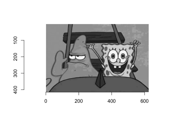
Okay, plenty of dirty math. It’s time to decompose our favorite Spongebob and Patrick.

Source

The first thing we need to do is to decolorize this picture, since a black-and-white picture could be represented as a matrix of numbers. Each number represents brightness of a pixel.

# load imager for plot pictures 
library(imager)

# load the picture, you may right click and save the picture to your local disc, if you want to follow the process
spongebob = load.image("spongebob.jpeg") 

# make spongebob grey
greyspongebob = grayscale(spongebob)

plot(greyspongebob)

Now we can convert the grey picture into a matrix, which has a dimension of 625 * 415

greyspongebob_mat = as.matrix(greyspongebob)
dim(greyspongebob_mat)

Time to decompose!

# use built-in function svd()
greyspongebob_svd = svd(greyspongebob_mat)

The result is a list with three elements:

greyspongebob_svd$u contains the matrix $\mathbf{U}$

greyspongebob_svd$v contains the matrix $\mathbf{V}$

greyspongebob_svd$d contains a vector of singular values, but you can easily convert them to $\mathbf{\Sigma}$ by calling the function diag(greyspongebob_svd$d)

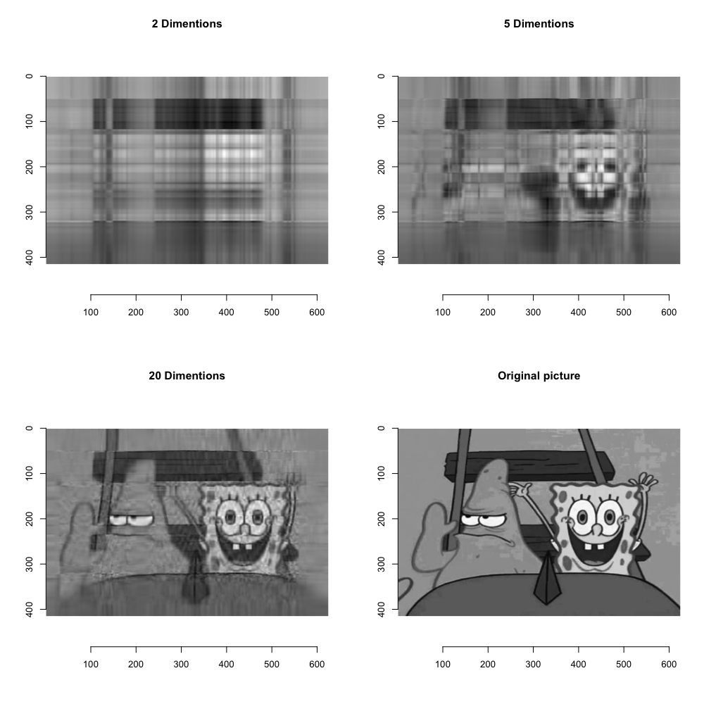
Now let’s re-construct the picture by selecting top-n dimensions. We write a function to make the job easier.

Reconstruct_Spongebob = function(dim){
  # reconstruct the matrix with top n dimentions
  mat = greyspongebob_svd$u[,1:dim] %*% diag(greyspongebob_svd$d[1:dim]) %*% t(greyspongebob_svd$v[,1:dim])
  
  # use imager package to redraw the picture
  mat %>% as.cimg(dim=dim(mat)) %>% plot(main=paste(dim, "Dimentions"))
}

Plot!

par(mfrow=c(2,2))
Reconstruct_Spongebob(2)
Reconstruct_Spongebob(5)
Reconstruct_Spongebob(20)
plot(greyspongebob, main = "Original picture")

As you can see, with 20 dimensions, we can reconstruct the picture reasonably well.

But think about how many space we need to use. $$ dim( \mathbf{U}) = 625 \times 20 = 12500 \\ dim( \mathbf{\Sigma}) = 20 \times 1 = 20 \\ dim( \mathbf{V}) = 415 \times 20 = 8300$$

In total, we need $12500 + 20 + 8300 = 20820$ numbers to represent the reduced picture.

However, we need $625 \times 415 = 259375$ numbers to represent the original picture! This is $10\times$ more than the reduced picture!

Okay, hope you find this post to be useful. If so, please don’t hesitate to give it a thumb up!