A random walk through HMM (2) - structure and inference
Introduction
I found most of HMM tutorial are presented in a top-down manner, where a lot of mathematical notations are thrown to the learners without a concrete example. This could sometimes make the learning process very frustrating, at least for me. In this post, I will try to demonstrate the core idea of HMM, as well as a commonly-used inference algorithm using a toy example. The example is from Dr.Xiaole Liu’s Youtube channel, and I highly recommend you to check out her video if you want to develop intuition of HMM rather than get killed by notations. Also, you may want to review conditional independence before you start reading, since a lot of derivations will use this property.
Set up the model
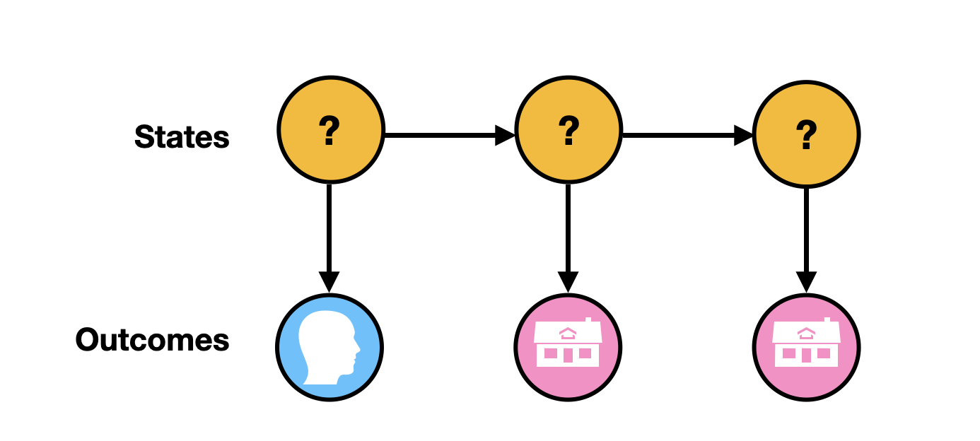
I have a biased coin and a fair coin. Each time I toss a coin under the table, and will show you the outcome (Head or Tail). After I toss this coin, There will be a chance that I will switch to a different coin or to continue to use the same coin, and make another toss under the table. Again, what you can see is the outcome of the coin toss, but you don’t know if I used a fair coin or a biased coin. Your job is to make an educated guess of which coin I have used to generate the sequence of outcomes. To make the example more concrete, imagine I tossed the coin three times, and the outcome is Head - Tail - Tail, as the diagram shows:
Besides the sequence of the outcome, you have another three pieces of information to help you make this educated guess:
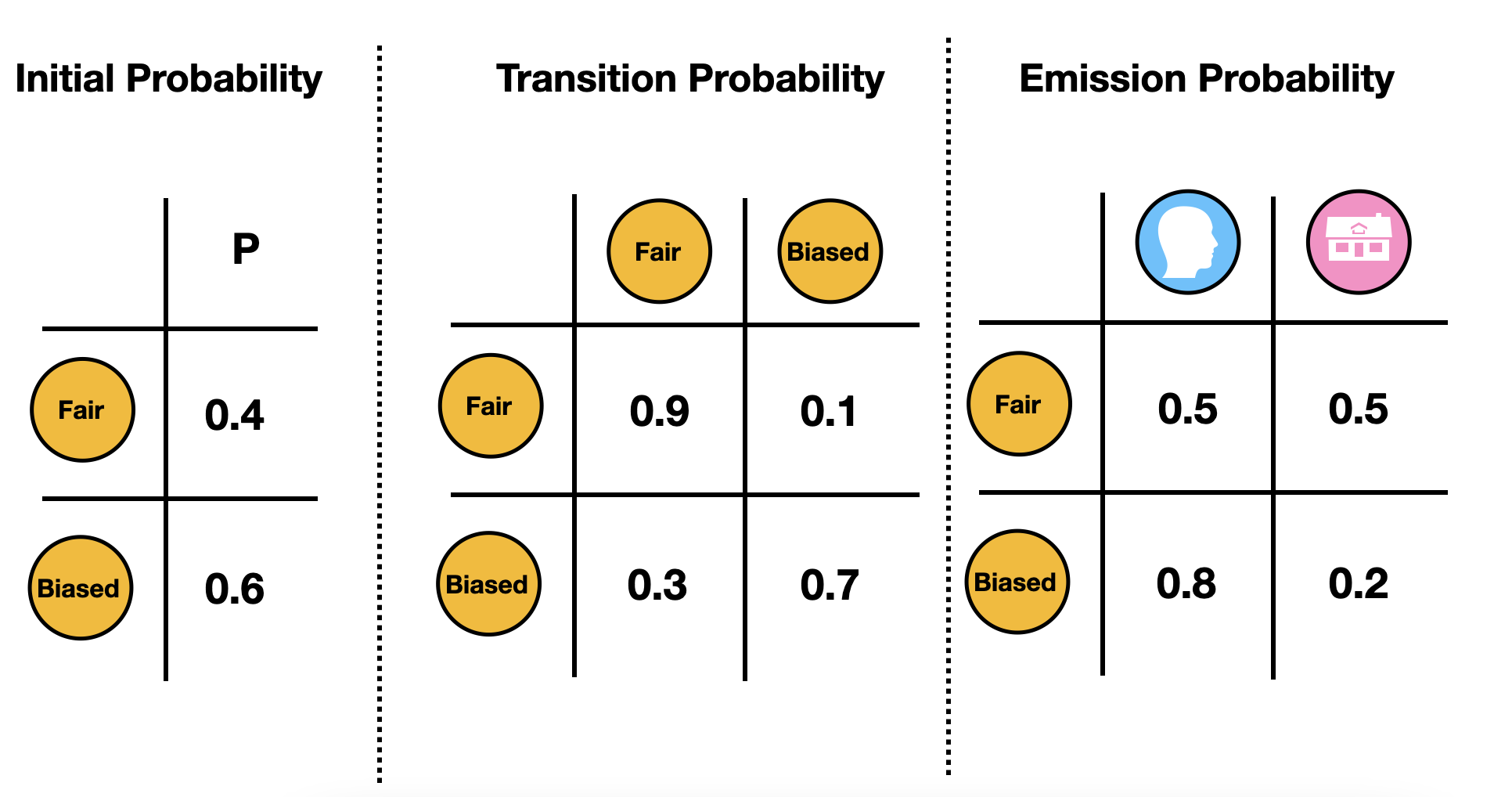
- Initial probability of which coin I used.
- Transition probability, meaning the probability that I switch from a Fair coin to a Biased coin, or vice versa. In the following graph, we are saying if I use a fair coin this time, then I have have 90% of chance to continue to use a fair coin, and 10% of chance to switch to a biased coin. If I used a biased coin this time, I will have 30% of chance to switch to a fair coin next time, and 70% of chance to use the same coin.
- Emission probability, meaning the probability of getting Head/Tail, given the coin is Fair/Biased. Here, we will have 50% of chance to get Head/Tail if I am using a fair coin. However, if I am using a biased coin, I will have 80% chance to get a head, and 20% chance to get a tail.
I think it’s important to first clarify some notations. Here is a few examples to help demonstrate:
The probability of getting a fair coin at the beginning (time 1) can be denoted as $P(F_1) = 0.4$
The probability of switching to a fair coin at time 3, given that we see a biased coin at time 2 can be denoted as $P(F_3 | B_2) = 0.3$
The probability of seeing a tail at time 2, given that we have a fair coin at time 2 can be denoted as $P(T_2 | F_2) = 0.5$
Brutal force inference
Before we jump into the detail, let me reiterate the goal: we want to guess the most possible sequence of states that generates the outcome. In our example, when did I use a fair coin and when did I use a biased coin.
Let’s first assume our coin sequence is Biased – Biased – Fair. The question is: what is the probability of seeing this coin sequence and the outcome sequence.
What we need to do here is simply multiply all the transition probability (including the initial probability of getting a biased coin) from Biased – Biased – Fair and their emission probability Biased – Head, Biased – Tail, Fair – Head.
$$ \begin{aligned} P(B_1, B_2, F_3, H_1, T_2, T_3) &= P(B_1) \cdot P(H_1 | B_1) \cdot P(B_2 | B_1)\cdot P(T_2 | B_2) \cdot P(F_3 | B_2)\cdot P(T_3 | F_3) \\ &= 0.6 \times 0.8 \times 0.7 \times 0.2 \times 0.3 \times 0.5 \\ & = 0.01008 \end{aligned} $$
Of course there are more than one way to get a sequence of Head – Tail – Tail. For example, to get Head – Tail – Tail, we can have our coin sequence to be Fair – Fair – Biased, Biased – Fair – Biased, etc. In fact there are $2^3= 8$ possible ways to get Head – Tail – Tail, and here is the table with their probabilities.
| Coin sequence | Probability of coin sequence and outcome sequence |
|---|---|
| $F_1, F_2, F_3$ | $P(F_1, F_2, F_3, H_1, T_2, T_3) = 0.0405$ |
| $F_1, F_2, B_3$ | $P(F_1, F_2, B_3, H_1, T_2, T_3) = 0.0018$ |
| $F_1, B_2, F_3$ | $P(F_1, B_2, F_3, H_1, T_2, T_3) = 0.0006$ |
| $F_1, B_2, B_3$ | $P(F_1, B_2, B_3, H_1, T_2, T_3) = 0.00056$ |
| $B_1, F_2, F_3$ | $P(B_1, F_2, F_3, H_1, T_2, T_3) = 0.0324$ |
| $B_1, F_2, B_3$ | $P(B_1, F_2, B_3, H_1, T_2, T_3) = 0.00144$ |
| $B_1, B_2, F_3$ | $P(B_1, B_2, F_3, H_1, T_2, T_3) = 0.01008$ |
| $B_1, B_2, B_3$ | $P(B_1, B_2, B_3, H_1, T_2, T_3) = 0.009408$ |
Here we have enumerated all possible states. If we sum up all the values in the above table, we can achieve the probability of observing this sequence of outcome: $$ \begin{aligned} P(H_1, T_2, T_3) &= P(F_1, F_2, F_3, H_1, T_2, T_3) + P(F_1, F_2, B_3, H_1, T_2, T_3) + … + P(B_1, B_2, B_3, H_1, T_2, T_3) \\ & = 0.0405 + 0.0018 + 0.0006 + 0.00056 + 0.0324 + 0.00144 + 0.01008 + 0.009408 \\ & = 0.096788 \end{aligned} $$
Using conditional probability, we can achieve $P(\text{coin sequence} |H_1, T_2, T_3)$. For example, we can calculate the probability of our outcome sequence is from Fair – Fair – Fair:
$$ \begin{aligned} P(F_1, F_2, F_3 |H_1, T_2, T_3) & = \frac{P(F_1, F_2, F_3 ,H_1, T_2, T_3) }{P(H_1, T_2, T_3)} \\ & = \frac{0.0405}{0.096788} \\ & = 0.418 \end{aligned} $$
That means there are 41.8% of the chance that the outcome sequence is from Fair – Fair – Fair.
To see the whole picture, let’s calculate the probability of every possible coin sequence, given we observed Head – Tail –Tail outcome sequence:
| Coin sequence | Probability of coin sequence given outcome sequence |
|---|---|
| $F_1, F_2, F_3$ | $0.0405/0.096788= 0.4184403 $ |
| $F_1, F_2, B_3$ | $0.0018/0.096788= 0.01859735 $ |
| $F_1, B_2, F_3$ | $0.0006/0.096788= 0.006199116 $ |
| $F_1, B_2, B_3$ | $0.00056/0.096788= 0.005785841 $ |
| $B_1, F_2, F_3$ | $0.0324/0.096788= 0.3347522 $ |
| $B_1, F_2, B_3$ | $0.00144/0.096788= 0.01487788 $ |
| $B_1, B_2, F_3$ | $0.01008/0.096788= 0.1041451 $ |
| $B_1, B_2, B_3$ | $0.009408/0.096788= 0.09720213 $ |
According to this table, the most likely coin sequence is Fair – Fair – Fair, which has 41.8% of the chance. So here is our final answer:
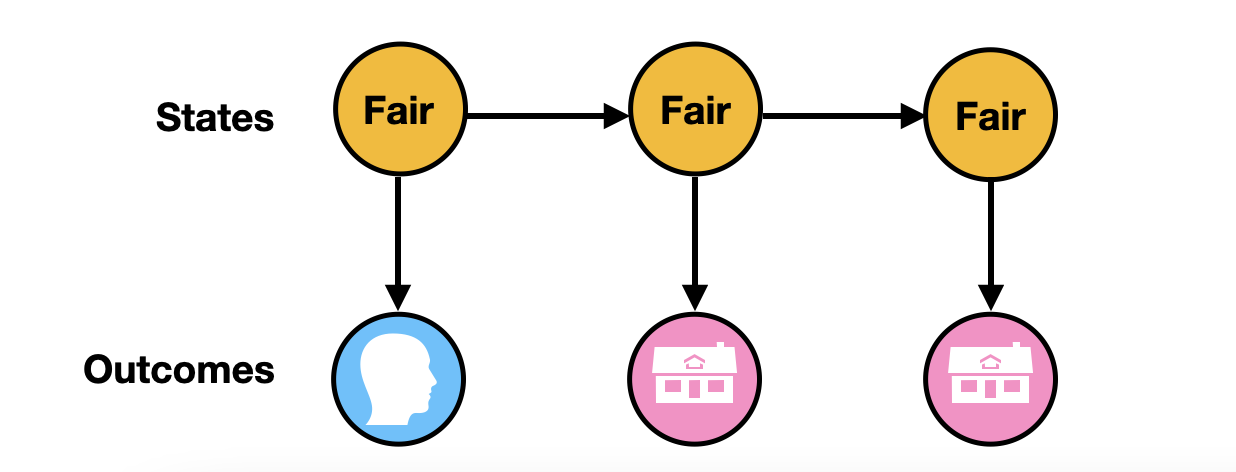
Besides inferring the coin sequence, we can also calculate the probability of head/tail at a given time. For example, we can calculate $P(F_2 |H_1, T_2, T_3 )$ by summing up all cases when the second coin is Fair, divided by all outcomes:
$$ \begin{aligned} P(F_2 |H_1, T_2, T_3 ) & = \frac{P(F_2 ,H_1, T_2, T_3) }{P(H_1, T_2, T_3)} \\ & = \frac{P(F_1, F_2, F_3,H_1, T_2, T_3) + P(F_1, F_2, B_3,H_1, T_2, T_3) + P(B_1, F_2, F_3,H_1, T_2, T_3) + P(B_1, F_2, B_3,H_1, T_2, T_3) }{P(H_1, T_2, T_3)} \\ & = \frac{0.0405 + 0.0018 + 0.0324 + 0.00144}{0.096788} \\ & = 0.7867 \end{aligned} $$
The results are telling us that we are 78% sure that the second toss is from a fair coin.
A drawback
The brutal force approach can help us develop intuition, but it should never be used to solve real-world problem. The biggest issue is the computation complexity. In our toy example, we have 3 observations, and we need to enumerate all $2^3 = 8$ cases in order to infer the hidden state. Imagine if we have 100 observations, we will have to enumerate all $2^{100}$ cases, which is never practical.
Forward Backward algorithm inference
I truly believe the guy who developed this method must be a genius. The beauty of this method is that we can infer the hidden states with a much lower computational complexity, and we can find the probability of Head/Tail at a given time point. The essence of this method is called dynamic programming, and I will demonstrate the idea below:
Forward algorithm
We first need to define a few quantities $\alpha_i(F)$ and $\alpha_i(B)$. It is the joint probability of all previously observed outcomes and the current state.
What do I mean by that? For example. $\alpha_2(F) = P(H_1, T_2, F_2)$. Similarly $\alpha_2(B) = P(H_1, T_2, B_2)$, $\alpha_3(B) = P(H_1, T_2,T_3, B_3)$, etc … (I hope the pattern is clear)
The quantities themselves might not be very interpretable, but a nice feature of this quantity is that each $\alpha$ can be derived from the previous $\alpha$. Let’s calculate them step by step:
Calculate $\alpha_1(F)$ and $\alpha_1(B)$:
$\alpha_1(F) = P(H_1, F_1) = P(F_1) \cdot P(H_1 |F_1) = 0.4 \times 0.5 = 0.2$
$\alpha_1(B) = P(H_1, B_1) = P(B_1) \cdot P(H_1 |B_1) = 0.6 \times 0.8 = 0.48$
Calculate $\alpha_2(F)$ and $\alpha_2(B)$:
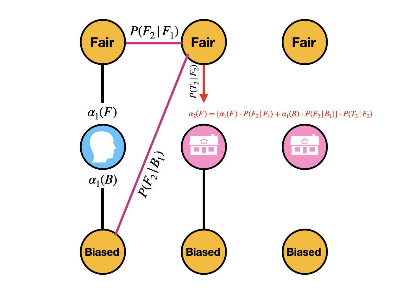
$$ \begin{aligned} \alpha_2(F) &= P(H_1, T_2, F_2) \\ &= [P(H_1, F_1, F_2) + P(H_1, B_1, F_2)] \cdot P(T_2 |F_2) \\ & = [P(H_1, F_1) \cdot P(F_2 |F_1) + P(H_1, B_1) \cdot P(F_2 |B_1)]\cdot P(T_2 |F_2) \\ & = [ \color{red} \alpha_1(F) \color{black} \cdot P(F_2 |F_1) + \color{red} \alpha_1(B) \color{black} \cdot P(F_2 |B_1)]\cdot P(T_2 |F_2) \\ & = (0.2 \times 0.9 + 0.48 \times 0.3)\times 0.5 \\ & = 0.162 \end{aligned} $$
$$ \begin{aligned} \alpha_2(B) &= P(H_1, T_2, B_2) \\ &= [P(H_1, F_1, B_2) + P(H_1, B_1, B_2)] \cdot P(T_2 |B_2) \\ & = [P(H_1, F_1) \cdot P(B_2 |F_1) + P(H_1, B_1) \cdot P(B_2 |B_1)]\cdot P(T_2 |B_2) \\ & = [ \color{red} \alpha_1(F) \color{black} \cdot P(B_2 |F_1) + \color{red} \alpha_1(B) \color{black} \cdot P(B_2 |B_1)]\cdot P(T_2 |B_2) \\ & = (0.2 \times 0.1 + 0.48 \times 0.7)\times 0.2 \\ & = 0.0712 \end{aligned} $$
I know the math is very messy, but here is a graphical demonstration of calculating $\alpha_2(F)$. It’s important to understand the pattern, and the same pattern can be applied to $\alpha_3(F)$ and $\alpha_3(B)$
Calculate $\alpha_3(F)$ and $\alpha_3(B)$:
Instead of deriving the formula from scratch, I will simply use the pattern above
$$ \begin{aligned} \alpha_3(F) & = P(H_1, T_2,T_3, F_3) \\ &= [ \color{red} \alpha_2(F) \color{black} \cdot P(F_3 |F_2) + \color{red} \alpha_2(B) \color{black} \cdot P(F_3 |B_2)]\cdot P(T_3 |F_3) \\ & = (0.162 \times 0.9 + 0.0712 \times 0.3) \times 0.5 \\ & = 0.08358 \end{aligned} $$
$$ \begin{aligned} \alpha_3(B) & = P(H_1, T_2,T_3, B_3) \\ &= [ \color{red} \alpha_2(F) \color{black} \cdot P(B_3 |F_2) + \color{red} \alpha_2(B) \color{black} \cdot P(B_3 |B_2)]\cdot P(T_3 |B_3) \\ & = (0.162 \times 0.1 + 0.0712 \times 0.7) \times 0.2 \\ & = 0.013208 \end{aligned} $$
I have color-coded the $\alpha$ in the equations. It’s important to notice that the next $\alpha$ can be derived from the previous $\alpha$ with the same pattern. It’s usage will be demonstrated in the next two sections.
Backward algorithm
Similar to $\alpha_i(F)$ and $\alpha_i(B)$, we will need to define another quantity called $\beta_i(F)$ and $\beta_i(B)$, which is the conditional probability of all the observations afterwards, given that the current coin is fair/biased. For example, $\beta_2(F) = P(T_3 |F_2)$, $\beta_1(B) = P(T_2, T_3 |B_1)$. Specifically, the last $\beta_i$, which is $\beta_3(F)$ and $\beta_3(B)$ in our example, is set to $1$.
I bet you will ask what is the point of defining this $\beta$ quantity. Please bare with me, it will be all clarified after I show you the mechanics.
Calculate $\beta_3(F)$ and $\beta_3(B)$:
As I said above, the last $\beta$ is set to $1$, so we have:
$\beta_3(F) = 1$
$\beta_3(B) = 1$
Calculate $\beta_2(F)$ and $\beta_2(B)$:
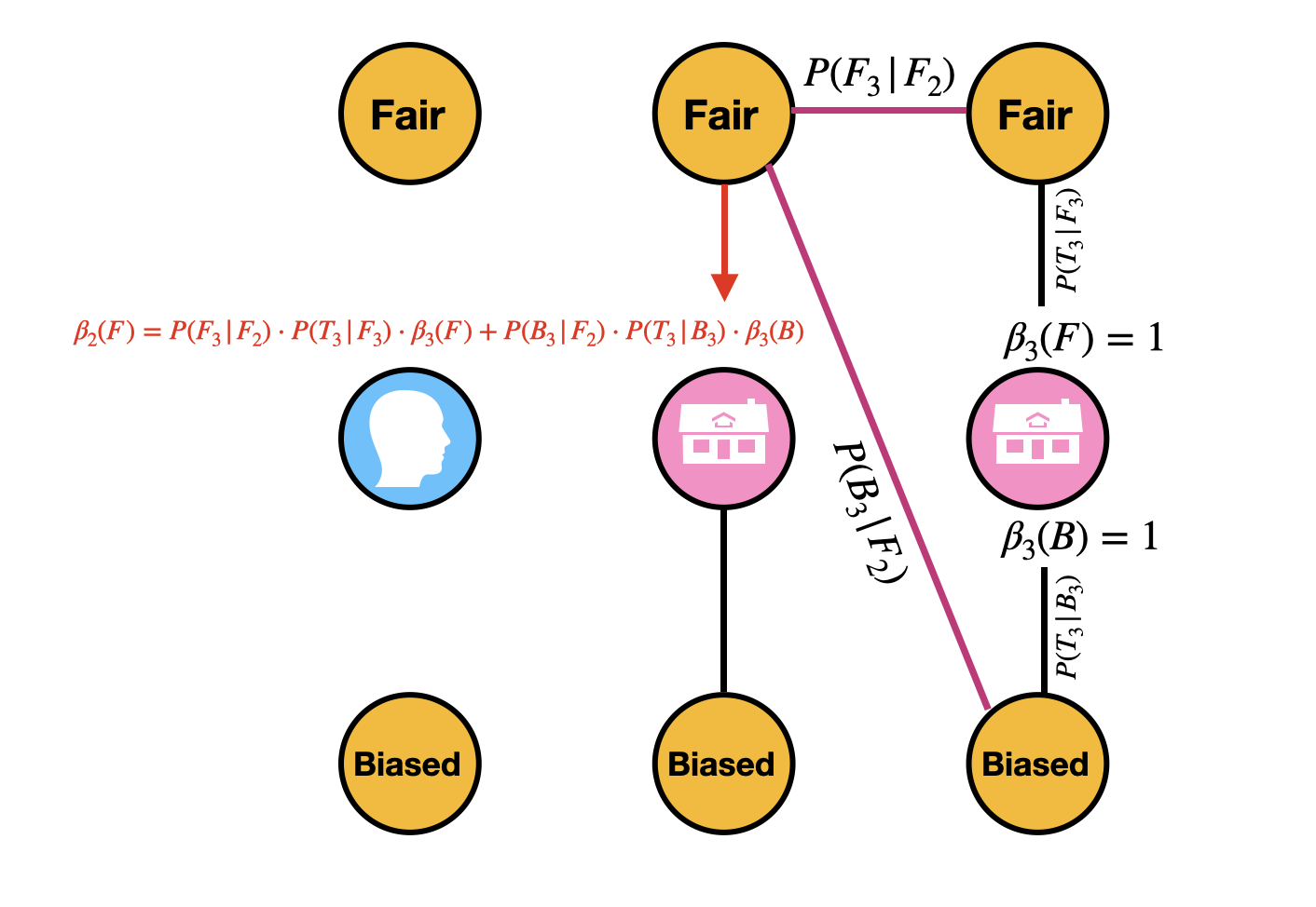
$$ \begin{aligned} \beta_2(F) & = P(T_3|F_2) \\ & = P(T_3, F_3 | F_2) + P(T_3, B_3 | F_2) \\ & = P(F_3 | F_2) \cdot P(T_3 | F_3) + P(B_3 | F_2) \cdot P(T_3 | B_3) \\ & = P(F_3 | F_2) \cdot P(T_3 | F_3) \cdot \color{red} \beta_3(F) \color{black} + P(B_3 | F_2) \cdot P(T_3 | B_3) \cdot \color{red} \beta_3(B) \color{black} \\ & = 0.9 \times 0.5 \times 1 + 0.1 \times 0.2 \times 1 \\ & = 0.47 \end{aligned} $$
$$ \begin{aligned} \beta_2(B) & = P(T_3|B_2) \\ & = P(T_3, F_3 | B_2) + P(T_3, B_3 | B_2) \\ & = P(F_3 | B_2) \cdot P(T_3 | F_3) + P(B_3 | B_2) \cdot P(T_3 | B_3) \\ & = P(F_3 | B_2) \cdot P(T_3 | F_3) \cdot \color{red} \beta_3(F) \color{black} + P(B_3 | B_2) \cdot P(T_3 | B_3) \cdot \color{red} \beta_3(B) \color{black} \\ & = 0.3 \times 0.5 \times 1 + 0.7 \times 0.2 \times 1 \\ & = 0.29 \end{aligned} $$
Again, the pattern of calculating $\beta$ is important.
Calculate $\beta_1(F)$ and $\beta_1(B)$:
$$ \begin{aligned} \beta_1(F) & = P(T_2, T_3|F_1) \\ & = P(F_2 | F_1) \cdot P(T_2 | F_2) \cdot \color{red} \beta_2(F) \color{black} + P(B_2 | F_1) \cdot P(T_2 | B_2) \cdot \color{red} \beta_2(B) \color{black} \\ & = 0.9 \times 0.5 \times 0.47 + 0.1 \times 0.2 \times 0.29 \\ & = 0.2173 \end{aligned} $$
$$ \begin{aligned} \beta_1(B) & = P(T_2, T_3|B_1) \\ & = P(F_2 | B_1) \cdot P(T_2 | F_2) \cdot \color{red} \beta_2(F) \color{black} + P(B_2 | B_1) \cdot P(T_2 | B_2) \cdot \color{red} \beta_2(B) \color{black} \\ & = 0.3 \times 0.5 \times 0.47 + 0.7 \times 0.2 \times 0.29 \\ & = 0.1111 \end{aligned} $$
Forward + backward
Here is a summary of all $\alpha$ and $\beta$ we have calculated:
| Quantity | $H_1$ | $T_2$ | $T_3$ |
|---|---|---|---|
| $\alpha(F)$ | 0.2 | 0.162 | 0.08358 |
| $\alpha(B)$ | 0.48 | 0.0712 | 0.013208 |
| $\beta(F)$ | 0.2173 | 0.47 | 1 |
| $\beta(B)$ | 0.1111 | 0.29 | 1 |
It turns out we can use $\alpha$ and $\beta$ to calculate another quantity $\gamma$, which represents the probability of having head/tail at that particular time point, given the observed data.
For example, let’s calculate $\gamma_2 (F)$
$$ \begin{aligned} \gamma_2 (F) & = P(F_2 |H_1, T_2, T_3 )\\ &= \frac{\alpha_2(F) \cdot \beta_2(F) }{\alpha_2(F) \cdot \beta_2(F) + \alpha_2(B) \cdot \beta_2(B)} \\ & = \frac{0.162 \times 0.47}{0.162 \times 0.47 + 0.0712 \times 0.29} \\ & = 0.7867 \end{aligned} $$
If you scroll up a little bit of this page, you should find this result is exactly the same as what we get using brutal force approach.
Let’s try to calculate the probability of having a fair/biased coin for every single time point:
| P | $H_1$ | $T_2$ | $T_3$ |
|---|---|---|---|
| Fair | 0.4490226 | 0.7866678 | 0.8635368 |
| Biased | 0.5509774 | 0.2133322 | 0.1364632 |
According to our final results table from forward-backward propagation, it looks like the hidden state is Biased – Fair – Fair, which is different from from our brutal force calculation. This is expected, since forward-backward algorithm tries to find the most likely state for any point of time, but it’s not meant to find the most likely sequence of states.
Lastly, I want to prove the following equation:
$$P(F_2 |H_1, T_2, T_3 ) = \frac{\alpha_2(F) \cdot \beta_2(F) }{\alpha_2(F) \cdot \beta_2(F) + \alpha_2(B) \cdot \beta_2(B)} $$
We have $$ \begin{aligned} P(F_2 |H_1, T_2, T_3 ) &= \frac{P(F_2 , H_1, T_2, T_3 )}{P(H_1, T_2, T_3)} \\ & = \frac{P(F_2 , H_1, T_2, T_3 )}{P(F_2 , H_1, T_2, T_3 ) + P(B_2 , H_1, T_2, T_3 )} \\ &= \frac{P(T_3 | H_1, T_2, F_2 ) \cdot P(H_1, T_2, F_2)}{P(T_3 | H_1, T_2, F_2 ) \cdot P(H_1, T_2, F_2) + P(T_3 | H_1, T_2, B_2 ) \cdot P(H_1, T_2, B_2)} \\ & = \frac{P(T_3 | F_2 ) \cdot P(H_1, T_2, F_2)}{P(T_3 | F_2 ) \cdot P(H_1, T_2, F_2) + P(T_3 | B_2 ) \cdot P(H_1, T_2, B_2)} \\ &= \frac{\beta_2(F) \cdot \alpha_2(F)}{\beta_2(F) \cdot \alpha_2(F) + \beta_2(B) \cdot \alpha_2(B)} \\ Q.E.D \end{aligned} $$
We have covered quite a lot of materials in this blog post. In the next blog post, I am planning to discuss viterbi algorithm, which is another greedy algorithm to infer the hidden states. Make sure to follow this series and leave comments if you have questions~
