Dive into Bayesian statistics (4): Posterior predictive distribution

2021-11-22 776 words 4 minutes

Contents

In the last few posts, we tried three methods (Integration, Conjugate Prior and MCMC) to infer the posterior distribution $P(\lambda | \text{data})$, which gave us

$$\lambda \sim \text{Gamma}(\alpha = 20, \beta = 6)$$

Now you may ask: Cool, we have our posterior distribution, but SO WHAT?

In this post, we are going to see why studying the posterior distribution is advantageous and interesting, and show you the internal relationship between a Poisson distribution, a Gamma distribution and a Negative binomial distribution.

Question:

Here is the data we have worked so far:

Time	Number of visitors
8:am - 9:am	5
9:am - 10:am	3
10:am - 11:am	4
11:am - 12:pm	6

In this post, we will try to answer a question: What is the probability that my website has no visitors in the next hour?

The question might look a little strange at the first glance. How am I supposed to know the number of visitors in the future? In this post, we are going to address this question in two different manners: a frequentist framework, and a Bayesian framework

A Frequentist Framework:

As what I have discussed in this post, we assumed that the data has a Poisson distribution, and used Maximum Likelihood Estimation to figure out the most likely $\lambda = 4.5$. Now, we can simply plug $\lambda = 4.5$ into the Poisson distribution formula, which becomes our inferred population now: $$ f(x) = \frac{4.5^x e^{-4.5}}{x!} $$

To answer the question above, we simply plug in $x = 0$, and get: $$ f(0) = \frac{4.5^0 e^{-4.5}}{0!} = 0.011 $$

So, under a frequentist framework, our answer is 0.011

A Bayesian Framework:

Now let’s try to answer the question using a Bayesian framework. We have already derived the posterior distribution:

$$\lambda \sim \text{Gamma}(\alpha = 20, \beta = 6)$$

Then we also have the distribution of the data:

$$x \sim \text{Poisson}(\lambda)$$

Let’s try to concatenate the gamma distribution (which is the pdf of $\lambda$), and the poisson distribution (which is the pdf of data). This should gives us the probability distribution of the predictive data.

$$ \begin{aligned} f(x; \alpha = 20, \beta = 6) & = \int_0^{+ \infty} \frac{\lambda^x e^{-\lambda}}{x!} \cdot \frac{6^{20}}{19!} \lambda^{19} e^{-6\lambda} \cdot d\lambda \\ & = \frac{6^{20}}{19! \cdot x!} \int_{0}^{+\infty} \lambda^{19 + x} e^{-7 \lambda} d\lambda \\ & \stackrel{\dagger}{=} \frac{6^{20}}{19! \cdot x!} \cdot \frac{\Gamma{(20 + x)}}{7^{20 + x}} \\ & = \frac{\Gamma (20 + x)}{19 ! \cdot x!} \cdot (\frac{6}{7})^{20} \cdot (\frac{1}{7})^x \\ & = \frac{\Gamma (20 + x)}{\Gamma (20) \cdot \Gamma (x + 1)} \cdot (\frac{6}{7})^{20} \cdot (\frac{1}{7})^x \\ & = {x + 19 \choose x}\cdot (\frac{6}{7})^{20} \cdot (\frac{1}{7})^x \end{aligned} $$

Note: step $\dagger$ holds because $$ \int_0^{+\infty} x^a e^{-bx} dx = \frac{ \Gamma(a + 1)}{b ^{a + 1}} \text{ ,where } a, b \text{ are integers} $$

Therefore, we can make the conclusion that the posterior predictive distribution has a negative binomial distribution with $p = 6/7, r = 20$

From the posterior predictive distribution, we can easily calculate the probability of having no visitors in the next hour:

$$ f(0) = {19 \choose 0}\cdot (\frac{6}{7})^{20} \cdot (\frac{1}{7})^0 = 0.046 $$

Sampling of posterior predictive

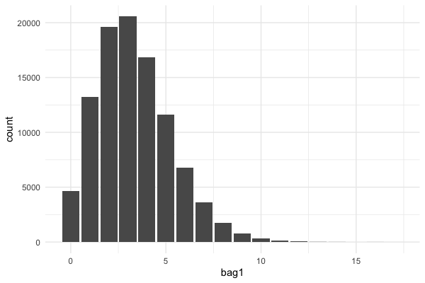
Lastly, let’s do a little bit of sampling to verify our result. Again, there are two ways:

Method 1:

Draw $\lambda$ from a gamma distribution, then use this lambda in a Poisson distribution:

library(ggplot2)
bag1 = c()

for (i in 1:100000){
  lambda = rgamma(1, shape = 20, rate = 6)
  bag1[i] = rpois(1, lambda = lambda)
}
# draw a histogram
ggplot(data.frame(bag1), aes(bag1)) + geom_bar()

This gave us:

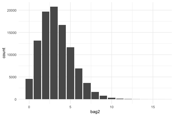
Method 2:

Draw samples from the negative binomial distribution directly:

bag2 = rnbinom(n = 100000, size = 20, prob = 6/7)
# draw a histogram
ggplot(data.frame(bag2), aes(bag2)) + geom_bar()

This gave us:

,which is almost identical as method 1

Summary:

In this post, we saw two completely different frameworks of inferring the data.

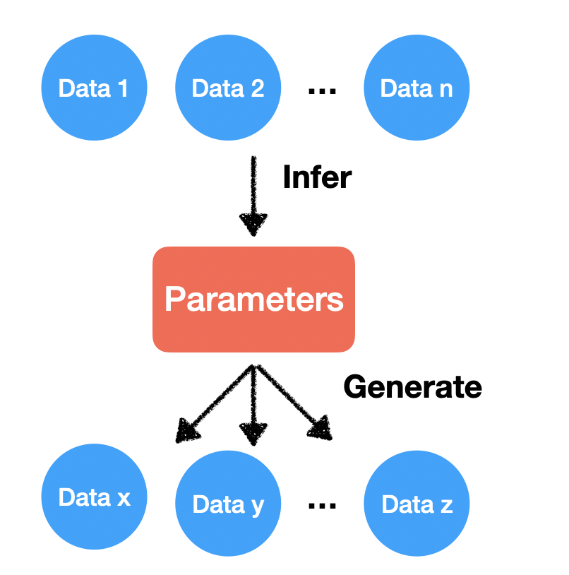
The frequentist approach assumes the parameters are fixed and data are random, and we use MLE to estimate the most likely parameters. Here is how it works:

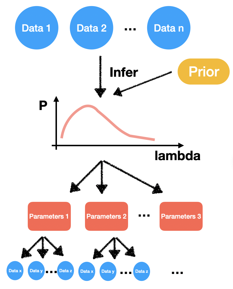
Whereas under the Bayesian framework, not only the data are random, but the parameters are also random. By adding a prior distribution, we can infer a parameter distribution. To generate data, we will first draw random parameters, and from those random parameters, we then draw random data. Here is a graphic demonstration: