Model the Gene Expression (1): A GLM framework
Before you start reading this post, please familiarize yourself with MLE and linear model.
Background
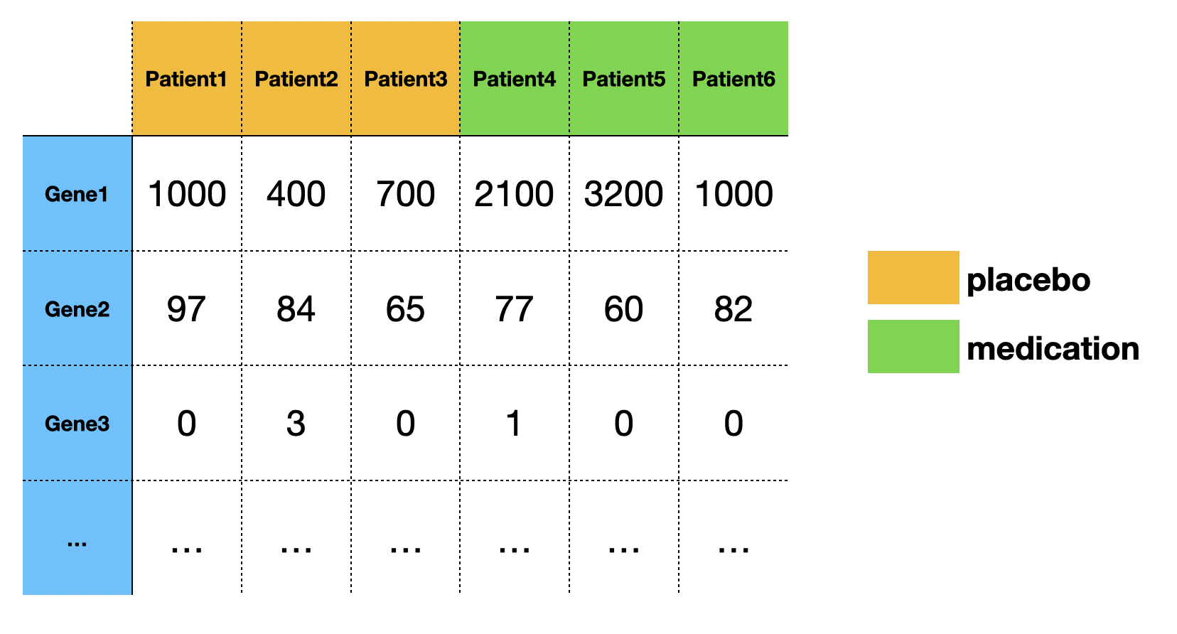
In transcriptomic research, we often want to determine if genes are unregulated or down-regulated under a particular perturbation. For example, we have a medication that may cure type 2 diabetes. In our experiment, 6 patients are split into two groups, with 3 patients taking the medication, and 3 patients taking the placebo. The patients' blood samples are then collected to measure the transcriptomic profile (mRNA abundance level for each gene) using NGS technology (RNA seq). The mRNA abundance levels are quantified by the number of reads that were mapped to the reference genome. Finally, we use statistical tests to determine if the level of change is big enough to be considered as a DEG (differentially expressed gene).
A typical RNA-seq experiment dataset (read counts) looks like:

In this post, we will only focus on one gene.
Negative Binomial Distribution
You might have noticed that in the table above, all the data is discrete counts. It is therefore inappropriate to use a normal distribution (a continuous distribution) to model the read counts. It is more common to use a Poisson distribution or a negative binomial distribution to model the gene expression in RNA-seq. For a Poisson distribution, it is assumed that the mean is equal to its variance, which isn’t true in most cases. The most accepted distribution among bioinformatics/biostatistics community is to use a negative binomial distribution, which allows us to model the data when its variance is much greater than its mean.
You might have seen that negative binomial distribution is formulated as: $$ \text{P(x = k)} = {k + n -1 \choose k}\cdot p^k \cdot (1-p)^n $$
This parameterization is advantageous when you want to model the number of failures before the experiment is stopped (e.g. how many times you need to flip a coin until you get 3 heads).
However, we would like to interpret our model in a more straightforward way. An alternative parameterization of negative binomial distribution is to use a mean parameter $\mu$, and a dispersion parameter $r$: $$ \text{P(x = k)} = \frac{\Gamma(r + k)}{k! \Gamma(r)} \cdot \Bigg( \frac{r}{r + \mu} \Bigg)^r \Bigg( \frac{\mu}{r + \mu} \Bigg)^k $$
, where the dispersion parameter $r = \frac{\mu^2}{\sigma^2 - \mu}$.
(Notice: in DESeq2, the dispersion parameter is written as $\alpha = \frac{\sigma^2 - \mu}{\mu^2}$, which is simply the reciprocal of $r$. We will stick with $r$, since the formula looks cleaner)
Warm up: fit a simple model
Let’s try to model the Gene1 expression level of patient1, patient2, patient3
| Patient | Gene1 Expression |
|---|---|
| patient1 | 1000 |
| patient2 | 400 |
| patient3 | 700 |
Technically, we should use Maximum Likelihood Estimation to estimate the parameters $r$, and $\mu$. The steps involve constructing a (log) likelihood function, taking the derivative, and finding $argmax$.
$$ \text{argmax}_{\mu, r} log \Bigg( P(y = 1000 |\mu, r) \cdot P(y = 400 |\mu, r) \cdot P(y = 700 |\mu, r) \Bigg) $$
,where $P(y_i |\mu, r) = \frac{\Gamma(r + y_i )}{y_i ! \Gamma(r)} \cdot \Big( \frac{r}{r + \mu} \Big)^r \Big( \frac{\mu}{r + \mu} \Big)^{y_i} $
(Note: the math could be very messy, and it’s impossible to find the analytical solution of the dispersion parameter $r$. We have to approximate $r$ by optimization approach like gradient descent)
Here is the R code implementation:
data = c(1000, 400, 700)
neg_loglikelihood = function(params){
  mu = params[1]
  r = params[2] # dispersion

  # define the log likelihood of each patient
  # patient 1-3 received placebo, therefore mu = b0
  loglikelihood1 = log(dnbinom(data[1], size = r, mu = mu))
  loglikelihood2 = log(dnbinom(data[2], size = r, mu = mu))
  loglikelihood3 = log(dnbinom(data[3], size = r, mu = mu))


  # summation of log, equivalent to log product.
  # optim function finds the minimum, we maximize the loglikelihood, which is equivalent to minimize neg_loglikelihood
  return(- (loglikelihood1 + loglikelihood2 + loglikelihood3))
}

# use optim to find argmin
optim(c(10,3), neg_loglikelihood)
You should get $$ \hat \mu = 700.444007 \\ \hat r = 7.635268 $$
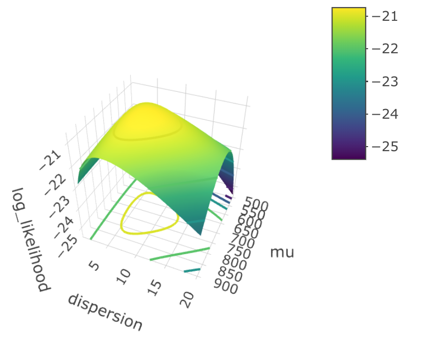
Here, I drew a 3D graph that shows you the relationship between log-likelihood, dispersion $r$ and mean $\mu$.

We can roughly tell that when $\hat \mu = 700$, $\hat r = 7.6$, the log likelihood function reach its maximum. These two values are so-called “population parameters”. Now, if we plug the estimated parameters into the formula, we have: $$ \text{P(x = k)} = \frac{\Gamma(7.6 + k)}{k! \Gamma(7.6)} \cdot \Bigg( \frac{7.6}{7.6 + 700} \Bigg)^{7.6} \Bigg( \frac{700}{7.6 + 700} \Bigg)^k $$
, and this is our fitted model.
Generalized Linear model
Now we need to take the effect of medication into our consideration. Keep in mind the independent variable is the medication/placebo, and the dependent variable is the expression level of Gene1.
| Patient | Treatment | Gene1 Expression |
|---|---|---|
| patient1 | placebo (0) | 1000 |
| patient2 | placebo (0) | 400 |
| patient3 | placebo (0) | 700 |
| patient4 | medication (1) | 2100 |
| patient5 | medication (1) | 3200 |
| patient6 | medication (1) | 1000 |
We will treat placebo as $0$, and medication as $1$.
We model the gene expression as
$$ y \sim NB(\mu, r) \\ log( \mu )= b_1 x + b_0 $$
It’s worth noticing that $b_1, b_0$, and $r$ are unknown, and the goal is to estimate them from our data.
The formula is confusing, isn’t it? Let’s plug in some numbers to see if the expression makes sense. Take patient1 as an example, we know patients 1 didn’t receive any medication, so we have $x_1 = 0$. $$ log(\mu_1) = b_1 \times 0 + b_0 \\ \mu_1 = e^{b_0} $$
Then we plug $\mu_1$ into the formula of negative binomial distribution: $$ NB(e^{b_0}, r ) $$
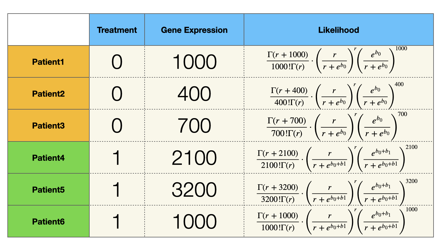
We observed the gene1 expression level for patient1, so we can formulate the likelihood function for patient1 as: $$ P(y_1 = 1000 |e^{b_0}, r ) = \frac{\Gamma(r + 1000)}{1000! \Gamma(r)} \cdot \Bigg( \frac{r}{r + e^{b_0}} \Bigg)^r \Bigg( \frac{e^{b_0}}{r + e^{b_0}} \Bigg)^{1000} $$
Similarly, we can express the likelihood function of all the patients:

Since samples (patients) are independently and identically distribution, the likelihood of observing all the patients is the product of the last column of the table above. $$ f(r, b_0, b_1) = \prod_{i = 1}^3 P(y_i |e^{b_0}, r ) \cdot \prod_{i = 4}^6 P(y_i |e^{b_0 + b1}, r ) $$
Notice the likelihood function $f(r, b_0, b_1)$ is a function of $r, b_0, b_1$, and we could use the same approach to find a set of parameters $\hat r, \hat b_0, \hat b_1$ that maximizes $f(r, b_0, b_1)$. Again, the actual calculation is tedious and unmanageable, and we should use optim() function to help us.
# observed data
data = c(1000, 400, 700, 2100, 3200, 1000)


neg_loglikelihood = function(params){
  b0 = params[1] # intercept
  b1 = params[2] # coefficient
  r = params[3] # dispersion

  # define the log likelihood of each patient
  # patient 1-3 received placebo, therefore mu = b0
  loglikelihood1 = log(dnbinom(data[1], size = r, mu = exp(b0)))
  loglikelihood2 = log(dnbinom(data[2], size = r, mu = exp(b0)))
  loglikelihood3 = log(dnbinom(data[3], size = r, mu = exp(b0)))

  # patient 4-6 received medication, therefore mu = b0 + b1
  loglikelihood4 = log(dnbinom(data[4], size = r, mu = exp(b0 + b1)))
  loglikelihood5 = log(dnbinom(data[5], size = r, mu = exp(b0 + b1)))
  loglikelihood6 = log(dnbinom(data[6], size = r, mu = exp(b0 + b1)))

  # summation of log, equivalent to log product.
  # optim function finds the minimum, we maximize the loglikelihood, which is equivalent to minimize neg_loglikelihood
  return(- (loglikelihood1 + loglikelihood2 + loglikelihood3 + loglikelihood4 + loglikelihood5 + loglikelihood6))
}


optim(c(5,2,3), neg_loglikelihood)
The optim function helped us find a set of parameters that maximize the loglikelihood function: $$\hat b_0 = 6.6 \\\ \hat b_1 =1.1 \\\ \hat r = 5.9$$
You might want to use glm.nb() function from the MASS package to fit the model. It should give us the same results
library(MASS)

# write data
data = c(1000, 400, 700, 2100, 3200, 1000)

# define group
expgroup = as.factor(c("control","control","control","treatment","treatment","treatment" ))

# build model
summary.glm(glm.nb(data ~ expgroup))
Summary
Generalized linear model is a very powerful approach that gives us more flexibility when linearity and normality don’t hold. Besides modeling the gene expression, GLM could also be used as a classification algorithm (logistic regression), which is something I will cover in the future.
Maximum likelihood estimation plays a critical role in GLM. It gives us a framework of estimating the population parameters, and helps us think probabilistically. In the next post, we will use MLE to perform hypothesis testing (likelihood ratio test). Stay tuned!
Reference
Wiki: https://en.wikipedia.org/wiki/Negative_binomial_distribution